Activation Functions Explained - GELU, SELU, ELU, ReLU and more

During the calculations of the values for activations in each layer, we use an activation function right before deciding what exactly the activation value should be. From the previous activations, weights and biases in each layer, we calculate a value for every activation in the next layer. But before sending that value to the activations of the next layer, we use an activation function to scale the output. Here, we will explore different activation functions.

The prerequisite for this post is my last post about feedforward and backpropagation in neural networks, you would have seen that I briefly talked about activation functions, but never actually expanded on what they do for us. Much of what I talk about here will only be relevant if you have the prior knowledge, or have read my previous post.

Neural Networks: Feedforward and Backpropagation Explained
What are neural networks? Developers should understand backpropagation, to figure out why their code sometimes does not work. Visual and down to earth explanation of the math of backpropagation.
Casper Hansen · Machine Learning From Scratch

Code > Theory? → Jump straight to the code.

Table of Contents (Click To Scroll)

0. Small Overview
1. What is the sigmoid function?
2. Gradient Problems: Backpropagation
   • Vanishing Gradients
   • Exploding Gradients
   • Extreme Example of Exploding Gradients
   • Avoiding Exploding Gradients: Gradient Clipping/Norms
3. Rectified Linear Unit (ReLU)
   • Dead ReLUs: The good and bad
4. Exponential Linear Unit (ELU)
5. Leaky Rectified Linear Unit (Leaky ReLU)
6. Scaled Exponential Linear Unit (SELU)
   • SELU: A special case of normalization
   • Weight Initialization + Dropout
7. Gaussian Error Linear Unit (GELU)
8. Code: Hyperparameter Search for Deep Neural Networks
9. Further Reading: Books and Papers

Small Overview

Activation functions can be a make-or-break-it part of a neural network. In this extensive article (>6k words), I'm going to go over 6 different activation functions, each with pros and cons. I will give you the equation, differentiated equation and plots for both of them. The goal is to explain the equation and graphs in simple input-output terms.

I show you the vanishing and exploding gradient problem; for the latter, I follow Nielsen's great example of why gradients might explode.

At last, I provide some code that you can run for yourself, in a Jupyter Notebook.

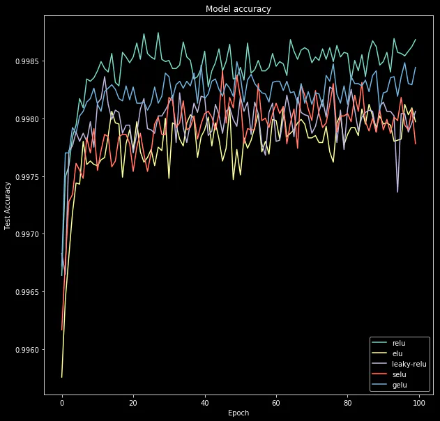
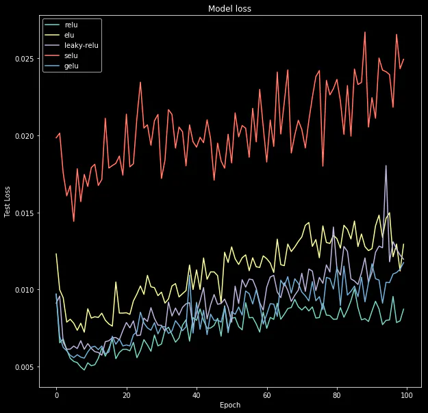
From the small code experiment on the MNIST dataset, we obtain a loss and accuracy graph for each activation function

Sigmoid function

The sigmoid function is a logistic function, which means that, whatever you input, you get an output ranging between 0 and 1. That is, every neuron, node or activation that you input, will be scaled to a value between 0 and 1.

$$\text{sigmoid}(x) = \sigma = \frac{1}{1+e^{-x}}$$

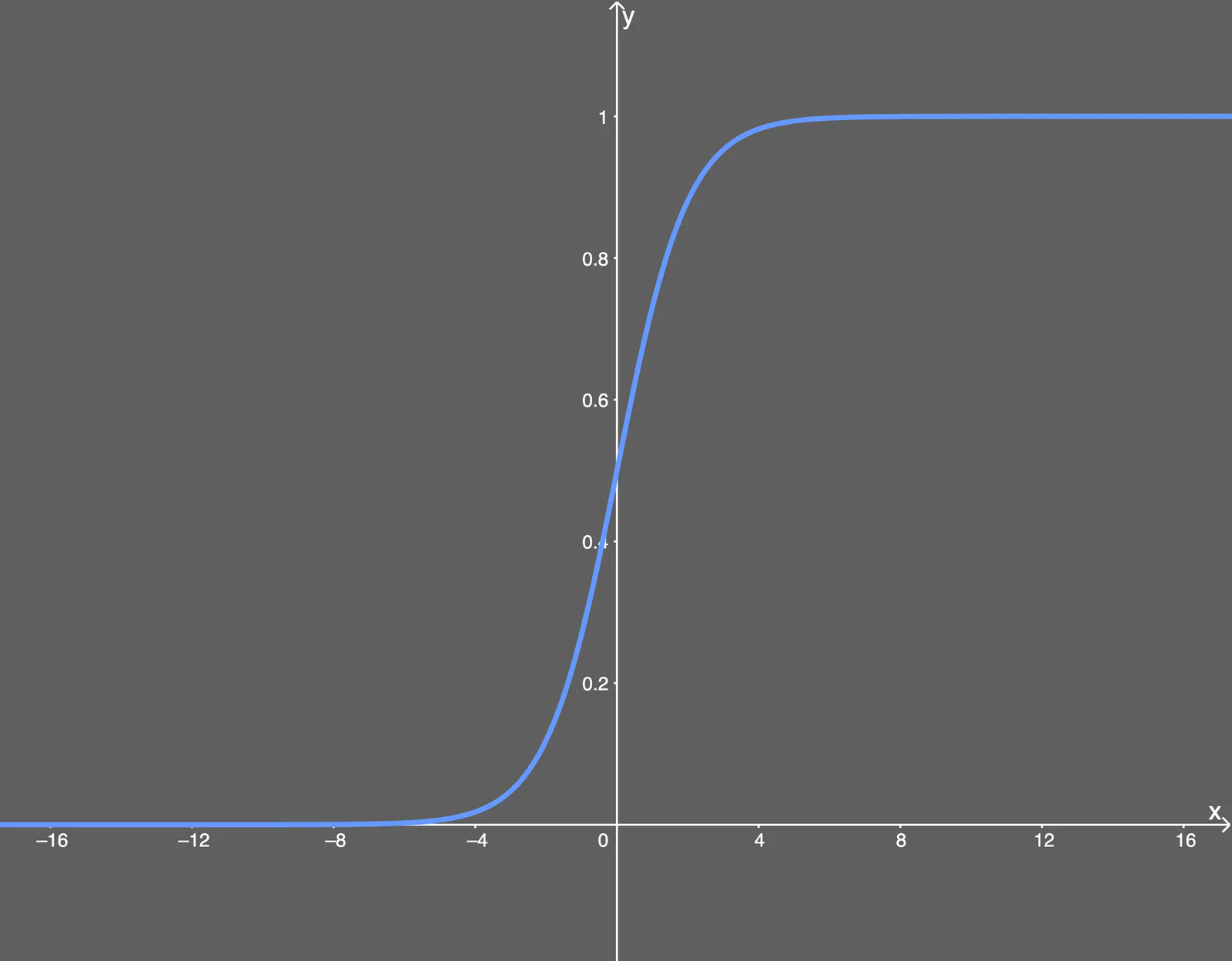
Sigmoid function plotted

Such a function, as the sigmoid, is often called a nonlinearity, simply because we cannot describe it in linear terms. Many activation functions are nonlinear, or a combination of linear and nonlinear – and it is possible for some of them to be linear, although that is unusual.

This is not entirely problematic, except for when the value gets very close to 0 or 1, which it will at some point. So why is this problematic?

This very question relates to backpropagation, covered here (read before continuing). In backpropagation, we calculate gradients for each weight, that is, small updates to each weight. We do this to optimize the output of the activation values throughout the whole network, so that it gives us a better output in the output layer, which in turn will optimize the cost function.

During backpropagation, we have to calculate the ratio of how much each weight impacts the cost function, by finding the partial derivatives of the cost function with respect to each weight. Let's say that we define all weights $w$ in the last layer $L$ by $w^L$, then the derivative of these will be, instead of defining individual weights

$$\frac{\partial C}{\partial w^{L}} = \frac{\partial C}{\partial a^{L}} \frac{\partial a^{L}}{\partial z^{L}} \frac{\partial z^{L}}{\partial w^{L}}$$

Note that when taking the partial derivative, we find the equation for $\partial a^{L}$ and then only differentiate $\partial z^{L}$, while the rest is constant. We denote the derivative of any function by an apostrophe '. When calculating the partial derivative for the middle term $\partial a^{L}/\partial z^{L}$, we get this

$$\frac{\partial a^{L}}{\partial z^{L}}= \sigma' \left( w \times a^{L-1}+b \right)$$

And the derivative of the sigmoid function turns out to be

$$\sigma'(x)=\sigma(x) (1-\sigma(x)) = \frac{e^{-x}}{(e^{-x}+1)^2}$$

When we input a large (positive or negative) $x$-value into the derivative of the sigmoid function, we get a $y$-value in return that is almost at 0 — that is, when we input $w \times a+b$, we might get a value close to zero in return.

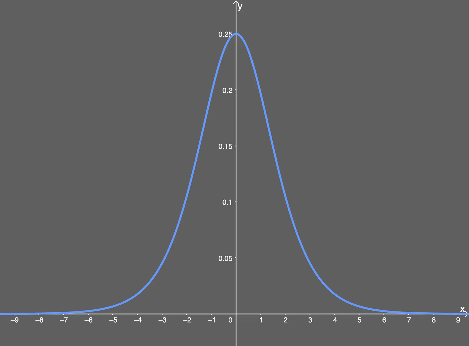
The derivative of the sigmoid function plotted as a graph

When $x$ is a large value (positive or negative), we essentially multiply a value that is almost zero with the rest of the partial derivatives.

$$\frac{\partial C}{\partial w^{L}} = \frac{\partial C}{\partial a^{L}} \times \text{almost zero} \times \frac{\partial z^{L}}{\partial w^{L}}$$

If enough weights have this behaviour of being a large value, we essentially get a network that does not adjust weights at all, which is a big problem. If we don't adjust the weights, we are left with the tiniest updates, which means that the algorithm does not improve the network much over time. For each of the calculations for partial derivatives with respect to a weight, we throw them into a gradient vector, which we use to update the neural network with. You might imagine, that if all the values of that gradient vector are close to zero, we are not really updating anything at all.

$$\sigma'(10)=\sigma(10)\times (1-\sigma(10)) = 0.00004539...$$

What has been described here is known as the vanishing gradient problem. Very briefly, this is why the sigmoid function should never be used over other activation functions, introduced later.

Vanishing Gradients Problem

Per my last post, if we want to update a specific weight, the update rule is

$$w^{(L)} = w^{(L)} - \text{learning rate} \times \frac{\partial C}{\partial w^{(L)}}$$

What if that partial derivative $\partial C/\partial w^{(L)}$ is vanishingly small? That is when we encounter the vanishing gradient problem, where a number of weights or biases essentially receive very small updates.

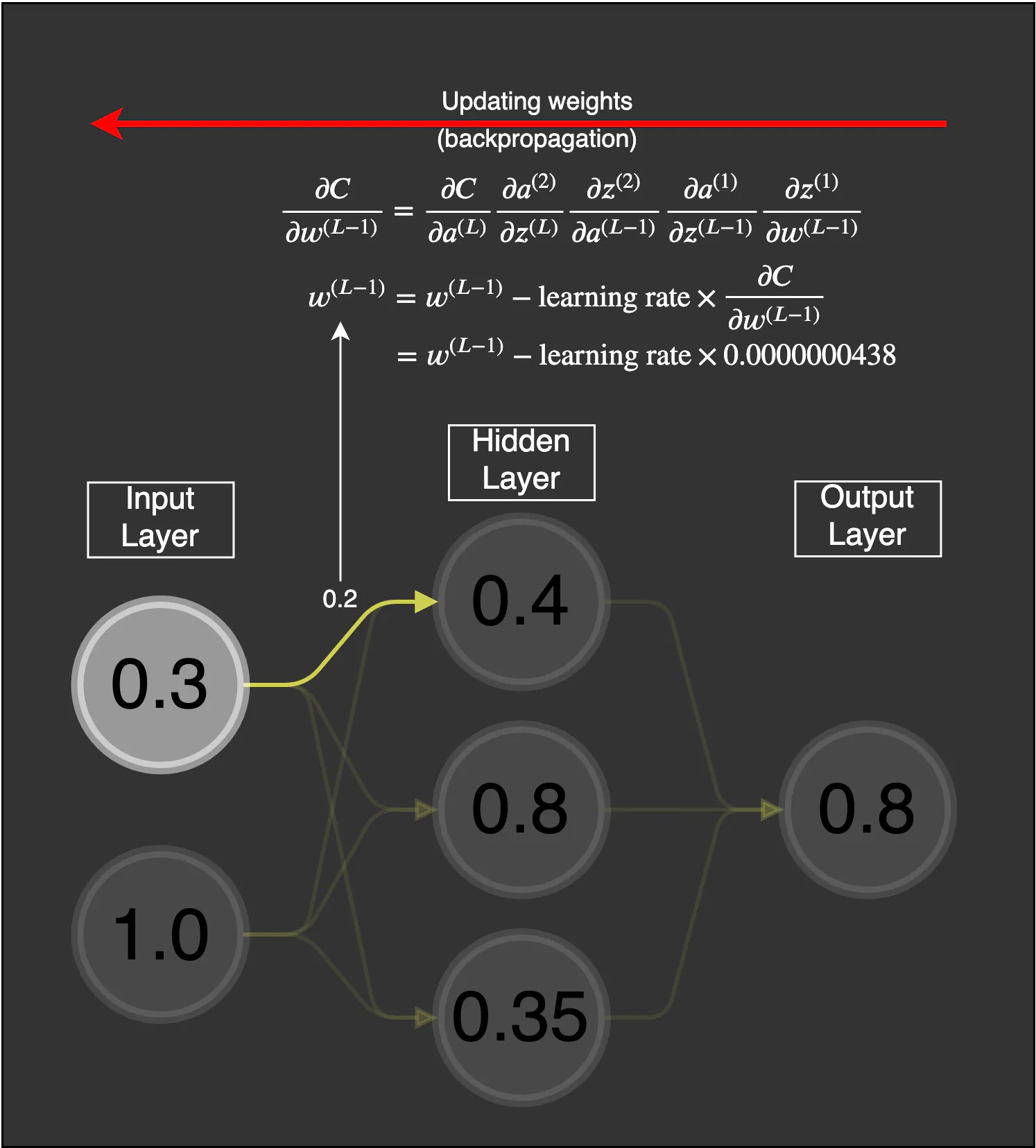
You see, if we have a weight with a value 0.2, it will barely move from that value if we have vanishing gradients. Since this weight is connecting the first neuron in the first layer and the first neuron in the second layer, we will call it $w^{(1)}_{1,1}$ in the notation of $w^{layer}_{to,from}$

$$w^{(1)}_{1,1}=w^{(1)}_{1,1}-\text{learning rate} \times 0.0000000438$$

Supposing that the weight has the value 0.2 and some given learning rate (doesn't matter, we will use 0.5), the new weight would be

$$w^{(1)}_{1,1}=0.2-0.5 \times 0.0000000438 = 0.199999978$$

The weight had the value $0.2$, but was updated to $0.199999978$. Evidently, this is a problem — gradients are vanishingly small and the weights in the neural networks will barely be updated. This causes nodes in the network to be far from their optimal value. This is a problem, that holds back a neural network from learning.

It has been observed that this becomes an even bigger problem, if you have different layers learning at different speeds. The layers will learn at different speeds, and the first layers will always be worse in the regard of learning rate.

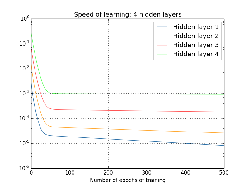
From Nielsen's book Neural Networks and Deep Learning

In this example, hidden layer 4 learns the fastest, because the cost function only depends on the changes of the weights connected to hidden layer 4. Let's consider hidden layer 1; here, the cost function depends on the changes of the weights connected to hidden layer 1 and hidden layer 2, 3 and 4's changes. If you followed my first post on backpropagation, maybe you picked up on the fact that earlier layers in the network reuse calculations from the later layers

$$\frac{\partial C}{\partial w^{(1)}} = \underbrace{ \frac{\partial C}{\partial a^{(4)}} \frac{\partial a^{(4)}}{\partial z^{(4)}} }_\text{From }w^{(4)} \, \underbrace{ \frac{\partial z^{(4)}}{\partial a^{(3)}} \frac{\partial a^{(3)}}{\partial z^{(3)}} }_\text{From }w^{(3)} \, \underbrace{ \frac{\partial z^{(3)}}{\partial a^{(2)}} \frac{\partial a^{(2)}}{\partial z^{(2)}} }_\text{From }w^{(2)} \, \frac{\partial z^{(2)}}{\partial a^{(1)}} \frac{\partial a^{(1)}}{\partial z^{(1)}} \frac{\partial z^{(1)}}{\partial w^{(1)}}$$

While, as shown earlier in this post, the last layer only depends on one set of changes when calculating partial derivatives

$$\frac{\partial C}{\partial w^{4}} = \frac{\partial C}{\partial a^{4}} \frac{\partial a^{4}}{\partial z^{4}} \frac{\partial z^{4}}{\partial w^{4}}$$

Ultimately, this is a big problem, because now the layers of weights are learning at a different rate. This means the later layers in the network will almost certainly be more optimized than the early layers in the network.

This is a problem, because the backpropagation algorithm doesn't know in which direction it should transform the weights, to optimize the cost function.

Exploding Gradients Problem

This problem is essentially the opposite of the vanishing gradient problem. It can be shown, as done by Nielsen, that we can get the opposite problem, where weights are essentially 'exploding' i.e. their values are rapidly increasing. We are going to be following his example here. Note that this can also be used to show the vanishing gradient problem, but I chose that problem to be more conceptual, for an easier explanation.

Essentially, we have the chance to run into a vanishing gradient problem when $0 < w < 1$ and an exploding gradient problem when $w > 1$. Though, for a layer to experience this problem, there must be more weights that satisfy the condition for either vanishing/exploding gradients.

---

We start off with a simple network. One which has few weights, biases and activations, and one which only has one node per layer.

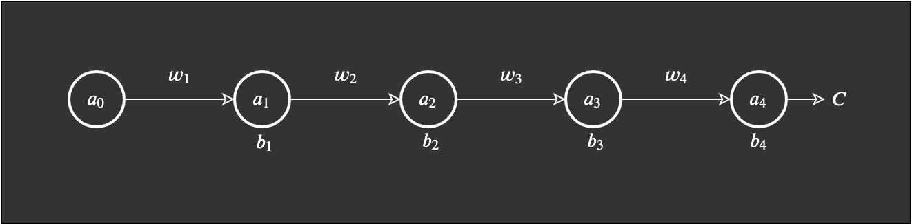
Simple; weights are indicated by $w_j$, biases $b_j$, with a cost function $C$. Nodes, neurons or activations (whatever you prefer) are the circles.

Nielsen uses a common notation from physics, describing change in some value, by the triangle symbol delta $\Delta$ (which is different from the gradient symbol nabla $\nabla$). For an example, $\Delta b_j$ is used to describe a change in the value for the j'th bias.

$$\Delta b_j = \text{how much }b_j\text{ changes}$$

The essence of my last post is that we measure the ratio of change in a weight or bias in relation to the cost function. Instead of considering a layer, let's focus on a specific bias, that is, the first bias $b_1$. Then we would measure the ratio by the equation

$$\frac{\partial C}{\partial b_1} = \frac{\partial C}{\partial a} \frac{\partial a}{\partial z} \frac{\partial z}{\partial b_1}$$

The argument for the next equation is the same as for the partial derivative above. That is, how do we measure a ratio of change in the cost function by the ratio of change in the bias?

As just described, Nielsen uses delta $\Delta$ to describe change so we could say that the partial derivatives could, roughly speaking, be replaced by delta

$$\frac{\partial C}{\partial b_1} \approx \frac{\Delta C}{\Delta b_1}$$

The changes to weights and biases can be visualized as follows:

GIF'ed from 3blue1brown video.

Let's start at the beginning of the network with calculating how a change in the first bias $b_1$ affects the network. Since we know, by my last post, that the first bias $b_1$ feeds into the first activation $a_1$, that is where we would start. Let's just recap to remind ourselves of the equation

$$a_1 = \sigma(z_1) = \sigma\left(w_1 a_0 + b_1 \right)$$

If $b_1$ changes, we call it $\Delta b_1$. Therefore, we notice that when $b_1$ changes, the activation $a_1$ also changes – which we normally express as $\partial a_1/\partial b_1$.

So we have the partial derivative expression on the left, which is the change in $a_1$ with relation to $b_1$. But then on the right side, we begin replacing terms, starting with replacing $a_1$ with the sigmoid of $z_1$

$$\frac{\partial a_1}{\partial b_1} = \frac{\partial \sigma(z_1) }{\partial b_1}$$

The above equation says that there is some change in the activation value $a_1$, when $b_1$ changes. Recall that we describe the change of $a_1$ as $\Delta a_1$.

We consider the change $\Delta a_1$ as being approximately the same as the rate of change of the activation value $a_1$ with respect to $b_1$ TIMES the change $\Delta b_1$

$$\begin{aligned} \Delta a_1 & \approx \frac{\partial \sigma(w_1 a_0+b_1)}{\partial b_1} \Delta b_1\\ & = \sigma'(z_1) \Delta b_1 \end{aligned}$$

We jumped over a step here, but essentially, we just calculated the partial derivative and replaced the fraction by the result of the partial derivative.

Changes in $a_1$ causes changes in $z_2$

The described change $\Delta a_1$ now causes a change in the input $z_2$ to the next layer. If this seems weird or you are not convinced, I encourage you to read through Neural Networks Explained.

$$z_2 = w_2 a_1 + b_2$$

Same notation as before, we call the next change $\Delta z_2$. The exact process we went through is used again, but this time to get to the change in $z_2$

$$\begin{aligned} \Delta z_2 & \approx \frac{\partial z_2}{\partial a_1} \Delta a_1\\ & = w_2 \Delta a_1 \end{aligned}$$

We could replace $\Delta a_1$ with the equation

$$\sigma'(z_1) \Delta b_1$$

We just calculated this equation. Hopefully it's clear how we got here – it's the same process we used to calculate $\Delta a_1$.

This process would just keep repeating until we have calculated the whole network. By replacing the $\Delta a_j$ values, we get a final function that calculates the change in the cost function with relation to the whole network – that is, all the weights, biases and activations

$$\begin{aligned} \Delta C & \approx \sigma'(z_1) w_2 \sigma'(z_2) \ldots \sigma'(z_4) \frac{\partial C}{\partial a_4} \Delta b_1 \end{aligned}$$

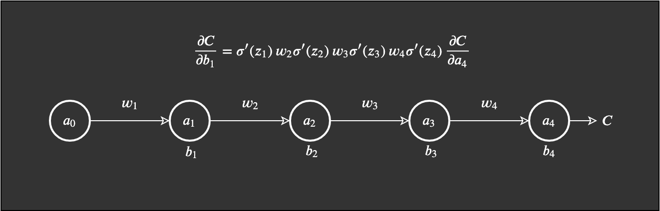
From this, we simply plug into the $\partial C/\partial b_1$ equation and get the final equation that we need

$$\begin{aligned} \frac{\partial C}{\partial b_1} = \sigma'(z_1) \, w_2 \sigma'(z_2) \, w_3 \sigma'(z_3) \, w_4 \sigma'(z_4) \, \frac{\partial C}{\partial a_4} \end{aligned}$$

Extreme Example

From here, what happens is that if all the weights $w_j$ all together are large, i.e. if many of the weights are equal to a value greater than 1, we start multiplying big values. For an example, say all weights have some extremely high value, like 100, and we get some random outputs of the derivative of the sigmoid function between 0 and 0.25:

$$\frac{\partial C}{\partial b_1} = 0.13 \times 100 \times 0.21 \times 100 \times 0.09 \times 100 \times 0.14 \frac{\partial C}{\partial a_4}$$

The last partial derivative turns out to be $2 \left(a_4 - y \right)$ for a squared error cost, which can be positive or negative, but for the sake of the example, we will set it equal to $-1$.

$$\begin{aligned} \frac{\partial C}{\partial b_1} & = 0.13 \times 100 \times 0.21 \times 100 \times 0.09 \times 100 \times 0.14 \times (-1)\\ & = -343.98 \end{aligned}$$

Using the update rule, and if we suppose $b_1$ previously was equal to $1.56$ and learning rate being equal to $0.5$

$$b_1 = 1.56 - 0.5 \times (-343.98) = 173.55$$

Although an extreme example, you get the point. The values for weights and biases can increasingly explode, causing the whole network to explode.

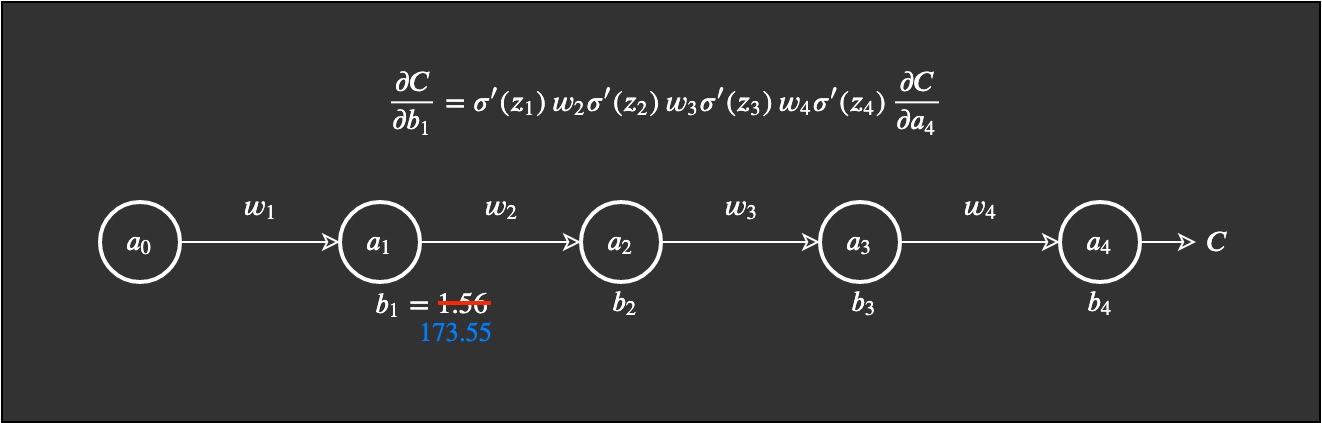
For a second, just imagine the rest of the network's weights and biases, and in turn activations, explosively updating their values. That is exactly what we call the exploding gradient problem. Obviously, the network won't learn much here, so this will completely ruin whatever task you are trying to solve.

Gradient Clipping/Norms

This idea is basically setting up a rule for avoiding exploding gradients. I won't go into the math on this one, but I will give you the steps on how it's done.

1. Pick a threshold value – if a gradient passes this value, gradient clipping or a gradient norm is applied.
2. Define if you are going to use gradient clipping or gradient norm. If gradient clipping, you specified a threshold value; e.g. 0.5. If the gradient value exceeds 0.5 or $-0.5$, then it will be either scaled back by the gradient norm or clipped back to the threshold value.

Note, however, that none of these gradient methods avoids the vanishing gradient problem. But we are going to further explore more options for that. Typically, you would need these kinds of methods, if you are using a Recurrent Neural Network architecture (like LSTM or GRU), since that is where you usually will experience exploding gradients.

ReLU

Rectified Linear Unit. This is how we fix the vanishing gradient problem, but does it cause other problems? Follow along.

This is the equation for ReLU:

$$\text{ReLU}(x)=\text{max}(0,x)$$

The ReLU equation tells us this:

1. If the input $x$ is less than 0, set the output equal to 0
2. If the input is greater than 0, set the output equal to the input

Although we can't exactly graph it with most tools, this is how you could explain the ReLU function in a graph. Everything with an x-value less than zero maps to a y-value of zero, but everything greater than zero is mapped to its own y-value. That is, if we input $x=1$, we get $y=1$ back.

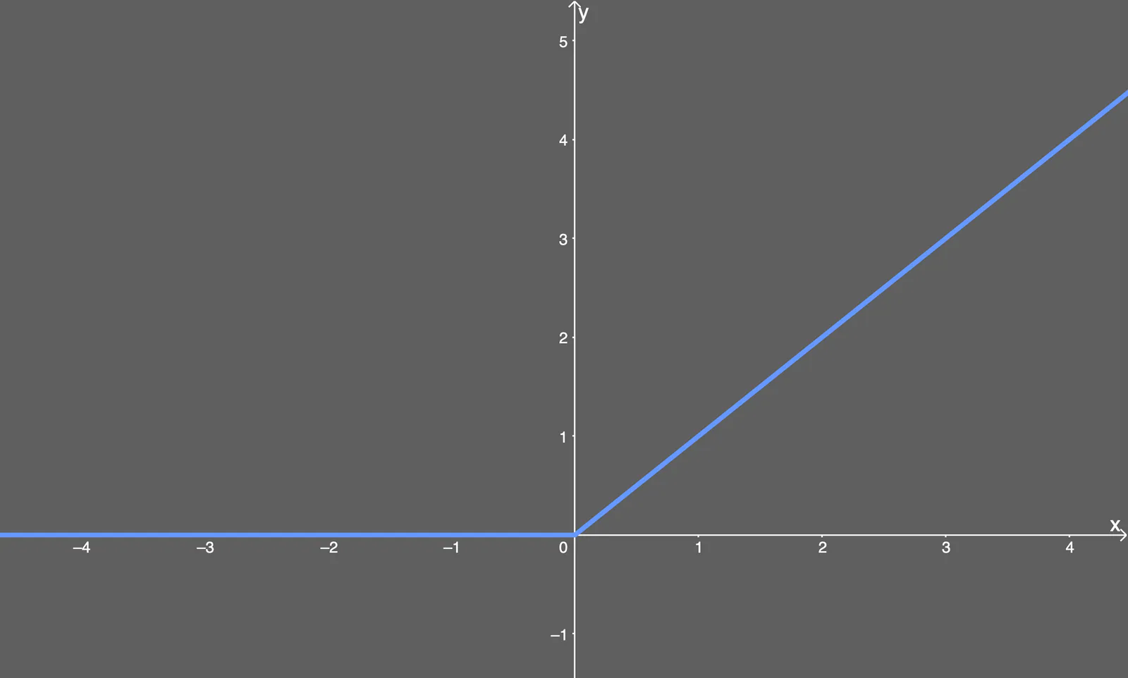
ReLU activation function plot

That's great, but how does that relate to the vanishing gradient problem? Firstly, we have to obtain the differentiated equation:

$$\text{ReLU}'(x) = \begin{cases} 1 & \mbox{if } x > 0\\ 0 & \mbox{if } x \leq 0 \end{cases}$$

This tells us that

1. If the input $x$ is greater than 0, then the output becomes 1
2. If the input is less than or equal (the $\leq$ symbol) to 0, then the output becomes 0

This is the graph for it

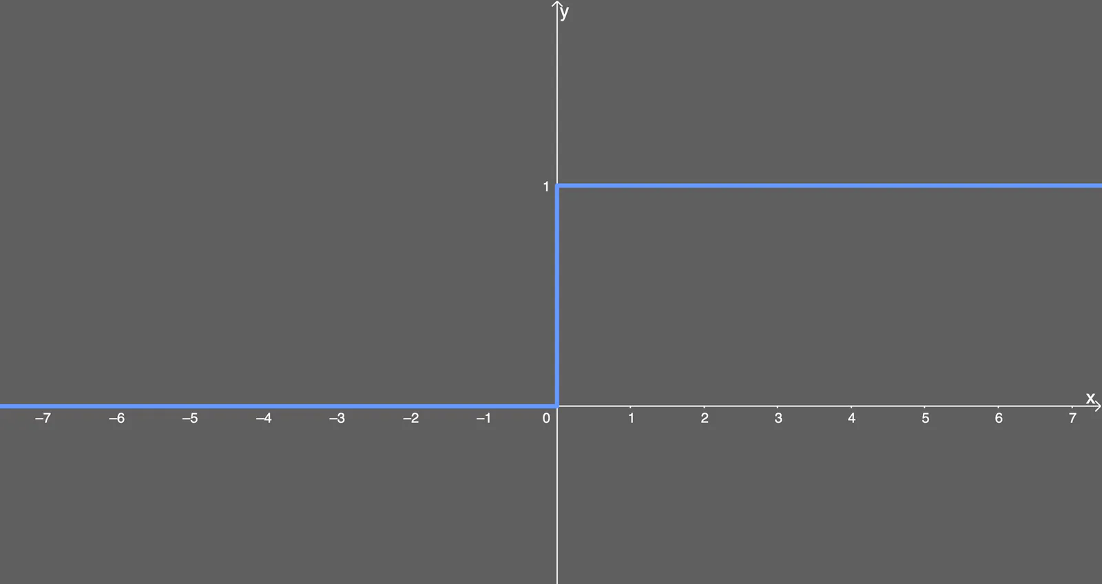
ReLU differentiated

Now we have the answer; we don't get extremely small values, when using a ReLU activation function — like $0.0000000438$ from the sigmoid function. Instead it's either 0, causing some of the gradients to return nothing, or 1.

This spawns another problem, though. The 'dead' ReLU problem.

What happens if too many values are below 0, when calculating gradients? We get a bunch of weights and biases that are not updated, since the update is equal to zero. To see this in action, let's reverse the exploding gradient example.

Let's denote ReLU as $R$ in this equation, where we just replaced every sigmoid $\sigma$ with $R$

$$\begin{aligned} \frac{\partial C}{\partial b_1} = R'(z_1) \, w_2 R'(z_2) \, w_3 R'(z_3) \, w_4 R'(z_4) \, \frac{\partial C}{\partial a_4} \end{aligned}$$

Now let's say a random $z$ input to the differentiated ReLU is less than 0 — the function will cause this bias to 'die'. Let's say it's $R'(z_3)=0$

$$\begin{aligned} \frac{\partial C}{\partial b_1} = R'(z_1) \, w_2 R'(z_2) \, w_3 0 \, w_4 R'(z_4) \, \frac{\partial C}{\partial a_4} \end{aligned} = 0$$

In turn, when we get that $R'(z_3)=0$, the rest of the values are multiplied and we get a whopping zero, which causes this bias to die. We know that the new value for the bias is the bias minus the learning rate times the gradient, which means we get an update of zero.

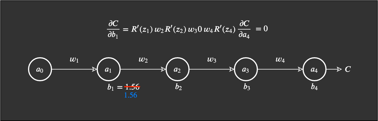
The good and the bad properties of dead ReLUs

When we introduce the ReLU function to a neural network, we also introduce great sparsity. Now what does this term sparsity actually mean?

Sparse: small in numbers or amount, often spread over a large area. In neural networks this means that the matrices for the activations have many $0$s. What do we obtain by this sparsity? When some percentage (e.g. 50%) of the activations are saturated, we would call the neural network sparse. This leads to an increase in efficiency with regards to time and space complexity – constant values (often) require less space and are less computationally expensive.

It has been observed by Glorot, Bordes and Bengio, that this component of ReLUs actually makes a neural network perform better, with the aforementioned efficiencies of time and space complexity.

Pros:

• Less time and space complexity, because of sparsity, and compared to the sigmoid, it does not involve the exponential operation, which is more costly.
• Avoids the vanishing gradient problem.

Cons:

• Introduces the dead relu problem, where components of the network are most likely never updated to a new value. This can sometimes also be a pro.
• ReLUs do not avoid the exploding gradient problem.

ELU

Exponential Linear Unit. This activation function fixes some of the problems with ReLUs and keeps some of the positive things. For this activation function, an alpha $\alpha$ value is picked; a common value is between $0.1$ and $0.3$.

The equation is a little more scary to look at, if you are not as much into math:

$$\text{ELU}(x) = \begin{cases} x & \mbox{if } x > 0\\ \alpha (e^x-1) & \mbox{if } x \leq 0 \end{cases}$$

Let me explain. If you input an x-value that is greater than zero, then it's the same as the ReLU – the result will be a y-value equal to the x-value. But this time, if the input value $x$ is less than 0, we get a value slightly below zero.

The y-value you get depends both on your x-value input, but also on a parameter alpha $\alpha$, which you can adjust as needed. Furthermore, we introduce an exponential operation $e^x$, which means the ELU is more computationally expensive than the ReLU.

The ELU function is plotted below with an $\alpha$ value of 0.2.

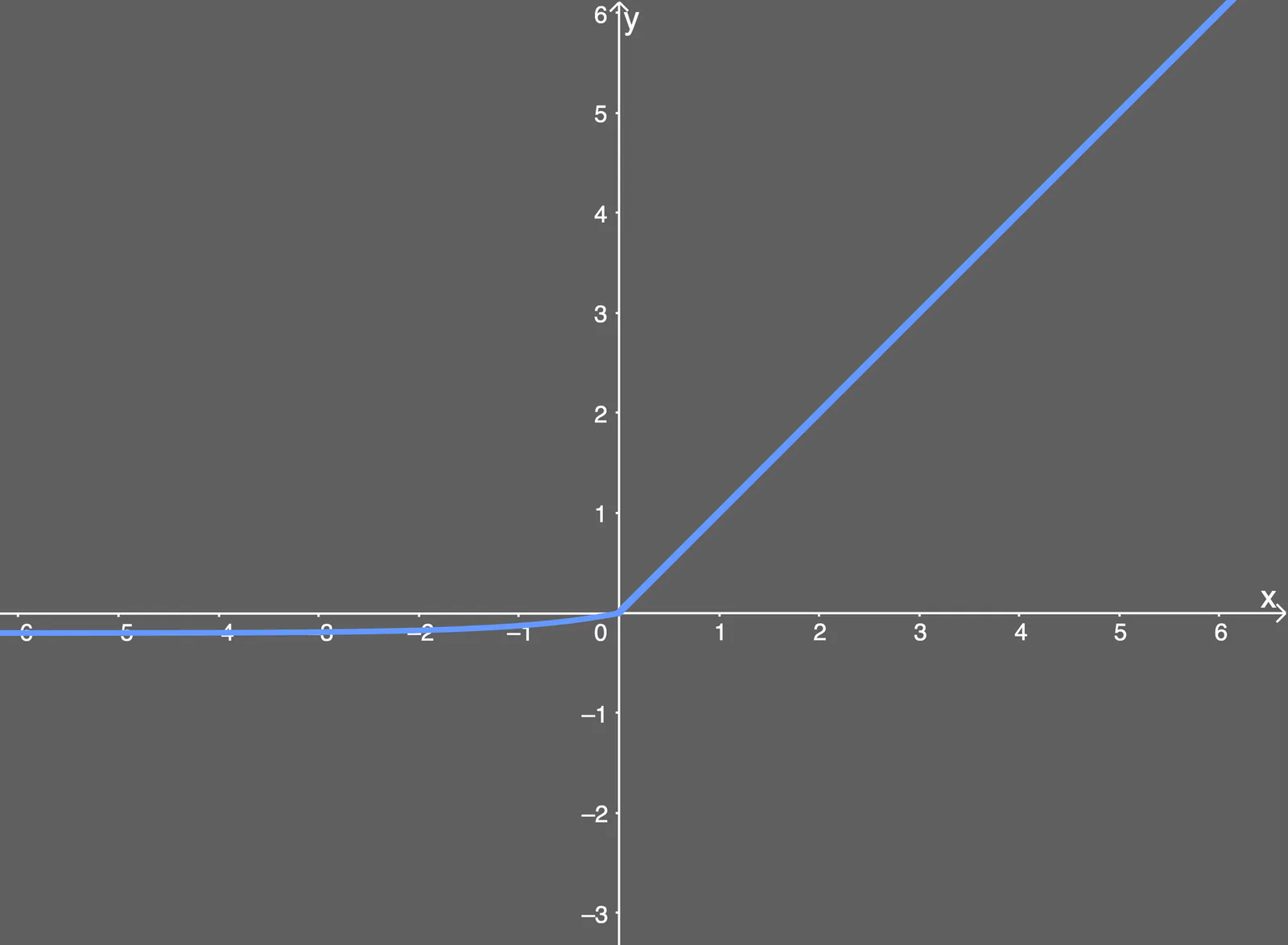
The plot for the ELU activation function

It's pretty straight forward, and we should still be good on the vanishing gradient problem, seeing as the input values don't map to extremely small output values.

But what about the derivative of the ELU? This is at least as important to show.

$$\text{ELU}'(x) = \begin{cases} 1 & \mbox{if } x > 0\\ \mbox{ELU}(x) + \alpha & \mbox{if } x \leq 0 \end{cases}$$

Seems simple enough. The y-value output is $1$ if $x$ is greater than 0. The output is the ELU function (not differentiated) plus the alpha value, if the input $x$ is less than zero.

The plot for it looks like this:

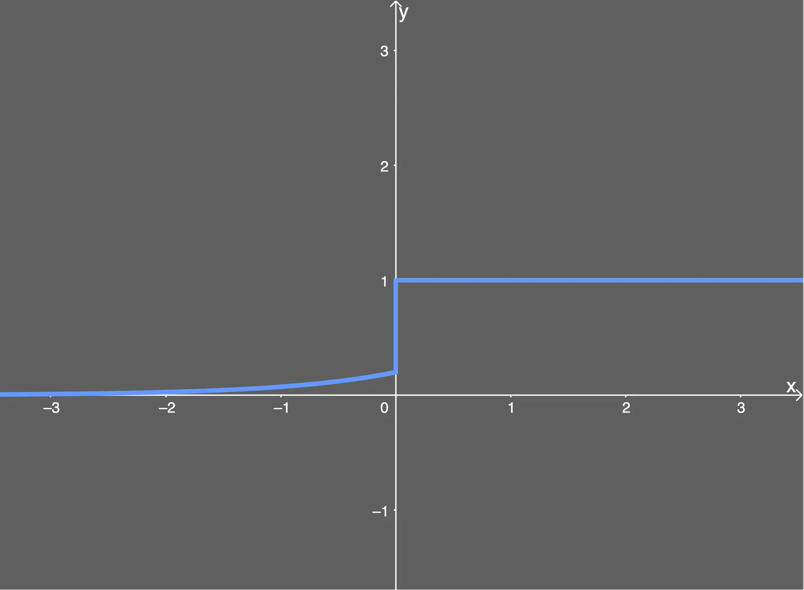
The ELU activation function differentiated

As you might have noticed, we avoid the dead relu problem here, while still keeping some of the computational speed gained by the ReLU activation function – that is, we will still have some dead components in the network.

Pros

• Avoids the dead relu problem.
• Produces negative outputs, which helps the network nudge weights and biases in the right directions.
• Produces activations instead of letting them be zero, when calculating the gradient.

Cons

• Introduces longer computation time, because of the exponential operation included
• Does not avoid the exploding gradient problem
• The neural network does not learn the alpha value

Leaky ReLU

Leaky Rectified Linear Unit. This activation function also has an alpha $\alpha$ value, which is commonly between $0.1$ and $0.3$. The Leaky ReLU activation function is commonly used, but it does have some drawbacks, compared to the ELU, but also some positives compared to ReLU.

The Leaky ReLU takes this mathematical form

$$\text{LReLU}(x) = \begin{cases} x & \mbox{if } x > 0\\ \alpha x & \mbox{if } x \leq 0 \end{cases}$$

So, if the input $x$ is greater than $0$, then the output is $x$. If the input is less than $0$, the output will be alpha $\alpha$ times the input.

This means that we solve the dead relu problem, because the values of the gradients can no longer be stuck at zero – also, this function avoids the vanishing gradient problem. Though an issue is that we still have to deal with exploding gradients, but more on how to prevent this later in the code section.

The Leaky ReLU is plotted here, with an assumption of alpha $\alpha$ being $0.2$:

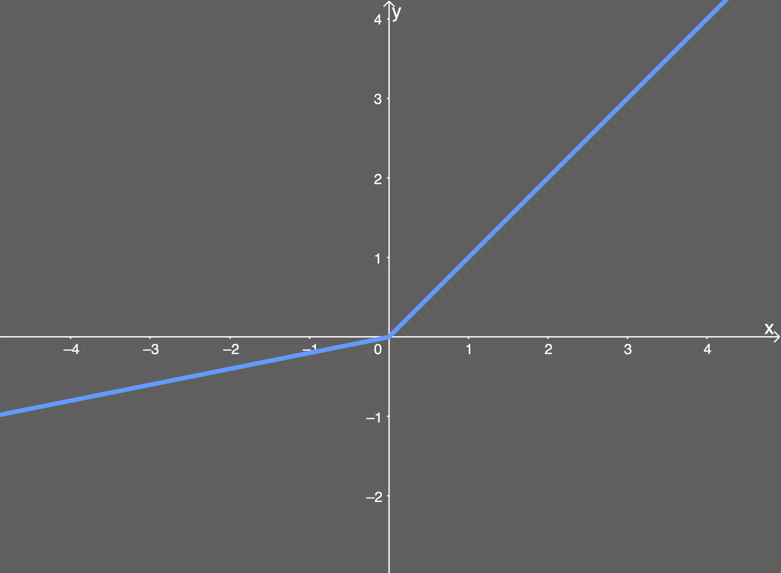
Leaky ReLU plotted

As explained from the equation, we see that any x-value maps to the same y-value, if the x-value is greater than $0$. But if the x-value is less than $0$, we have a coefficient of alpha, which is $0.2$. That means, if the input value $x$ is $-5$, the output value it maps to is $-1$.

Now, the derivative of the Leaky ReLU function is a bit simpler, as it entails two linear cases.

$$\text{LReLU}'(x) = \begin{cases} 1 & \mbox{if } x > 0\\ \alpha & \mbox{if } x \leq 0 \end{cases}$$

The first linear case is when the input $x$ is greater than $0$, then the output will be $1$. But if the input is less than $0$, then the output will be the value of alpha, which we chose to be $0.2$ in this instance.

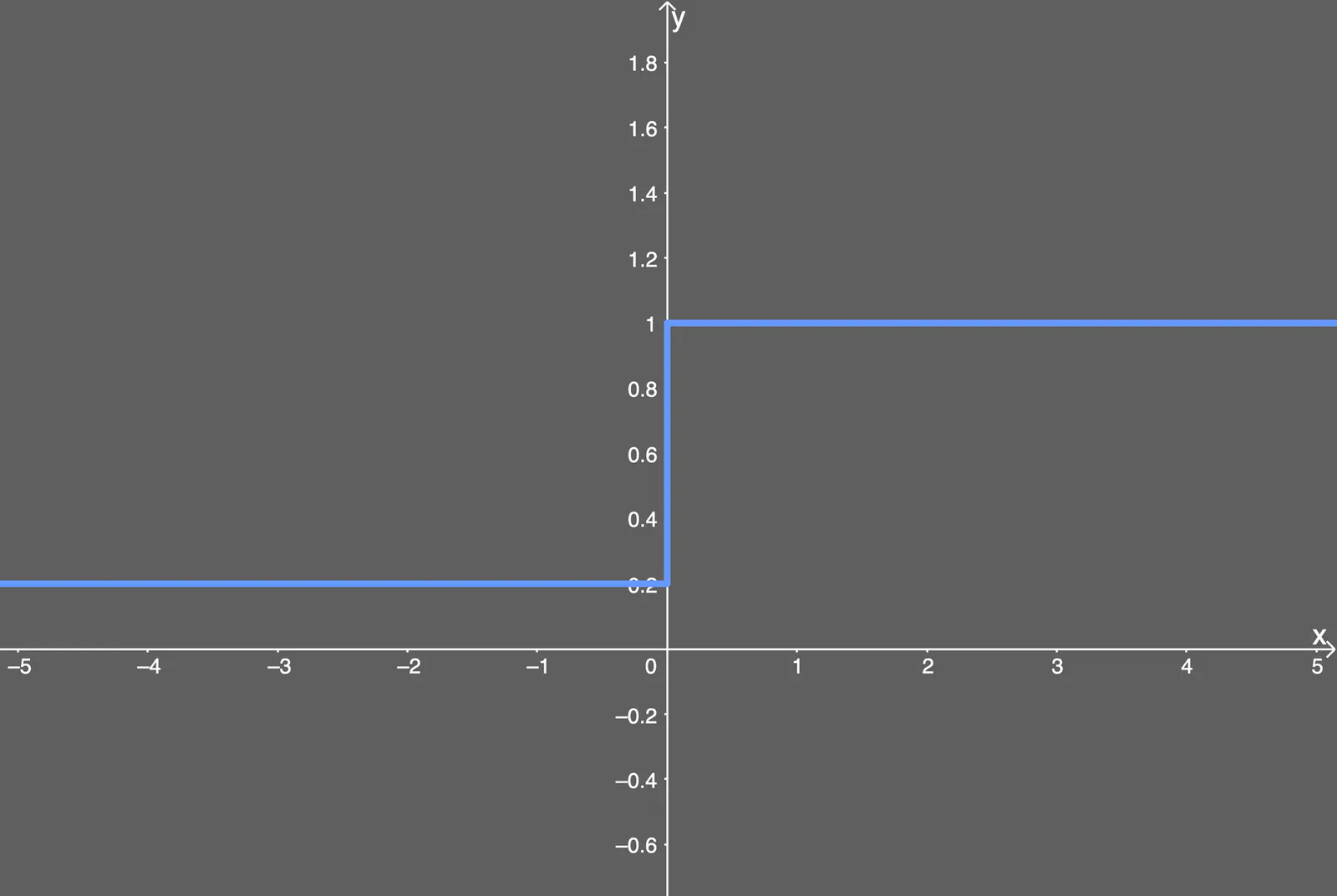
Differentiated Leaky ReLU plot

Notice how the function just becomes linear when differentiated – either $x$ is greater than zero and we get an output value of $1$, or $x$ is less than zero and we get an output value of alpha $\alpha$, which we chose to be $0.2$

Pros

• Like the ELU, we avoid the dead relu problem, since we allow a small gradient, when computing the derivative.
• Faster to compute than ELU, because no exponential operation is included

Cons

• Does not avoid the exploding gradient problem
• The neural network does not learn the alpha value
• Becomes a linear function, when it is differentiated, whereas ELU is partly linear and nonlinear.

SELU

Scaled Exponential Linear Unit. This activation function is one of the newer ones, and it comes with a particularly long appendix (90 pages) with theorems, proofs etc. When using this activation function in practice, one must use lecun_normal for weight initialization, and if dropout wants to be applied, one should use AlphaDropout. More on this later in the code section.

The authors have calculated two values; an alpha $\alpha$ and lambda $\lambda$ value for the equation, which I'm going to show first

$$\alpha \approx 1.6732632423543772848170429916717$$ $$\lambda \approx 1.0507009873554804934193349852946$$

They have that many numbers after the decimal point for absolute precision, and they are predetermined, which means we do not have to worry about picking the right alpha value for this activation function.

To be honest, the equation just looks like the other equations, which it more or less is. All the newer activation functions just look like a combination of the other existing activation functions.

The equation for it looks like this:

$$\text{SELU}(x) = \lambda \begin{cases} x & \mbox{if } x > 0\\ \alpha e^x-\alpha & \mbox{if } x \leq 0 \end{cases}$$

That is, if the input value $x$ is greater than zero, the output value becomes $x$ multiplied by lambda $\lambda$. If the input value $x$ is less than or equal to zero, we have a function that goes up to $0$, which is our output $y$, when $x$ is zero. Essentially, when $x$ is less than zero, we multiply alpha with the exponential of the x-value minus the alpha value, and then we multiply by the lambda value.

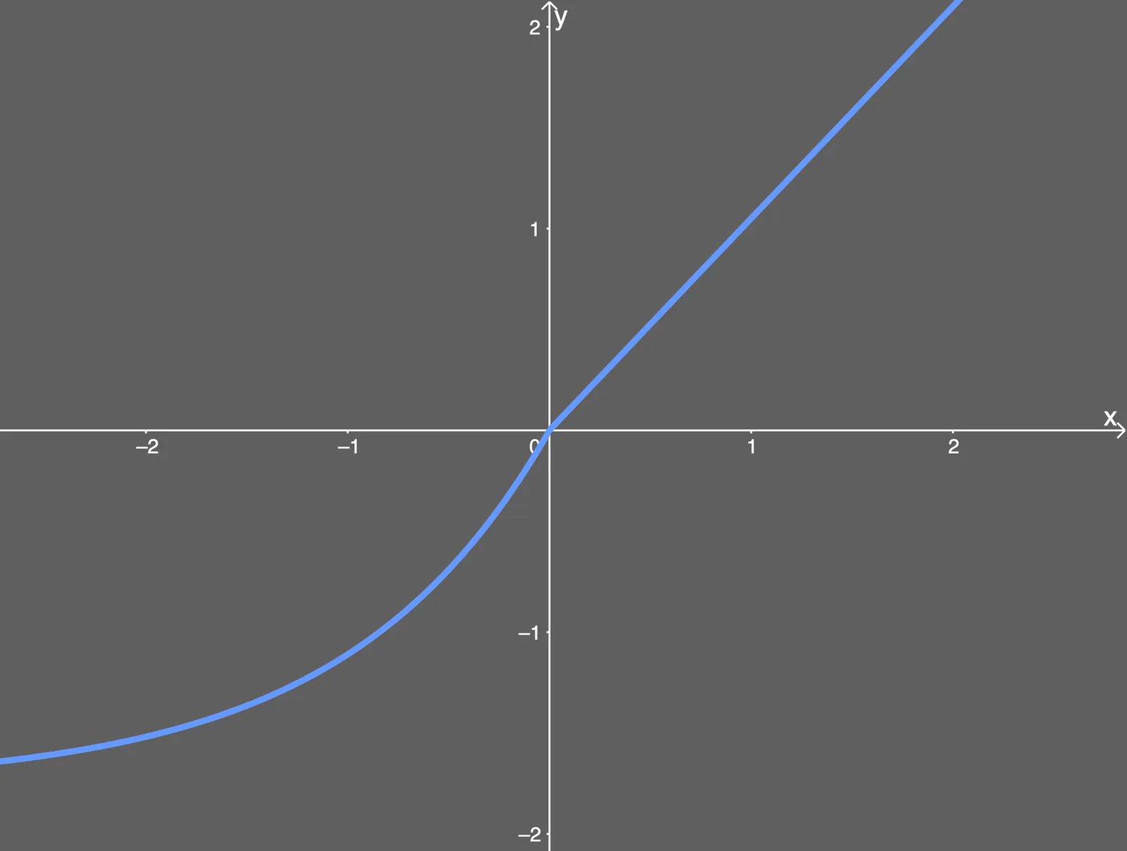
The SELU function plotted

The Special Case for SELU

The SELU activation is self-normalizing the neural network; and what does that mean?

Well, let's start with, what is normalization? Simply put, we first subtract the mean, then divide by the standard deviation. So the components of the network (weights, biases and activations) will have a mean of zero and a standard deviation of one after normalization. This will be the output value of the SELU activation function.

What do we achieve by mean of zero and standard deviation of one? Under the assumption, that the initialization function lecun_normal initializes the parameters of the network as a normal distribution (or Gaussian), then the case for SELU is that the network will be normalized entirely, within the bounds described in the paper. Essentially, when multiplying or adding components of such a network, the network is still considered to be a Gaussian. This is what we call normalization. In turn, this means that the whole network and its output in the last layer is also normalized.

How a normal distribution looks with a mean $\mu$ of zero and a standard deviation $\sigma$ of one.

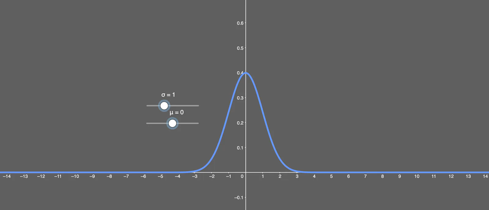
The output of a SELU is normalized, which could be called internal normalization, hence the fact that all the outputs are with a mean of zero and standard deviation of one, as just explained. This is different from external normalization, where batch normalization and other methods are used.

Okay, great, the components are normalized. But how does it actually happen?

The simple explanation is that variance decreases when the input is less than zero, and variance increases when the input is greater than zero – and the standard deviation is the square root of variance, so that is how we get to a standard deviation of one.

We get to a mean of zero by the output values of the activation function, where we need some positive and some negative, to be able to shift the mean to zero. Unlike the ReLU, whose outputs are never negative, the SELU can output negative values, which is what makes it possible to control the mean.

The main point of the mean mu $\mu$ and variance nu $\nu$, is that we have some domain omega $\Omega$, where we always map the mean and variance within predefined intervals. These intervals are defined as follows:

$$\text{mean} = \mu \in \left[ -0.1,\, 0.1 \right]$$ $$\text{variance} = \nu \in \left[ 0.8,\, 1.5 \right]$$

The $\in$ symbol just means that the mean or variance is within those predefined intervals. In turn, this causes the network to avoid vanishing and exploding gradients.

I want to quote from the paper, one which I find important and how they got to this activation function:

SELUs allow to construct a mapping g with properties that lead to SNNs [self-normalizing neural networks]. SNNs cannot be derived with (scaled) rectified linear units (ReLUs), sigmoid units, tanh units, and leaky ReLUs. The activation function is required to have (1) negative and positive values for controlling the mean, (2) saturation regions (derivatives approaching zero) to dampen the variance if it is too large in the lower layer, (3) a slope larger than one to increase the variance if it is too small in the lower layer, (4) a continuous curve. The latter ensures a fixed point, where variance damping is equalized by variance increasing. We met these properties of the activation function by multiplying the exponential linear unit (ELU) [7] with $\lambda > 1$ to ensure a slope larger than one for positive net inputs.

Let's move onto how the differentiated function looks like. Here it is:

$$\text{SELU}'(x) = \lambda \begin{cases} 1 & \mbox{if } x > 0\\ \alpha e^x & \mbox{if } x \leq 0 \end{cases}$$

Well.. nothing too fancy, that we can't explain with simple words. If $x$ is greater than zero, then the output value will be $\lambda$. But if $x$ is less than zero, then the alpha value is simply multiplied by the exponential operation on $x$, and then by $\lambda$.

The plot is seen as below, and it looks very unique.

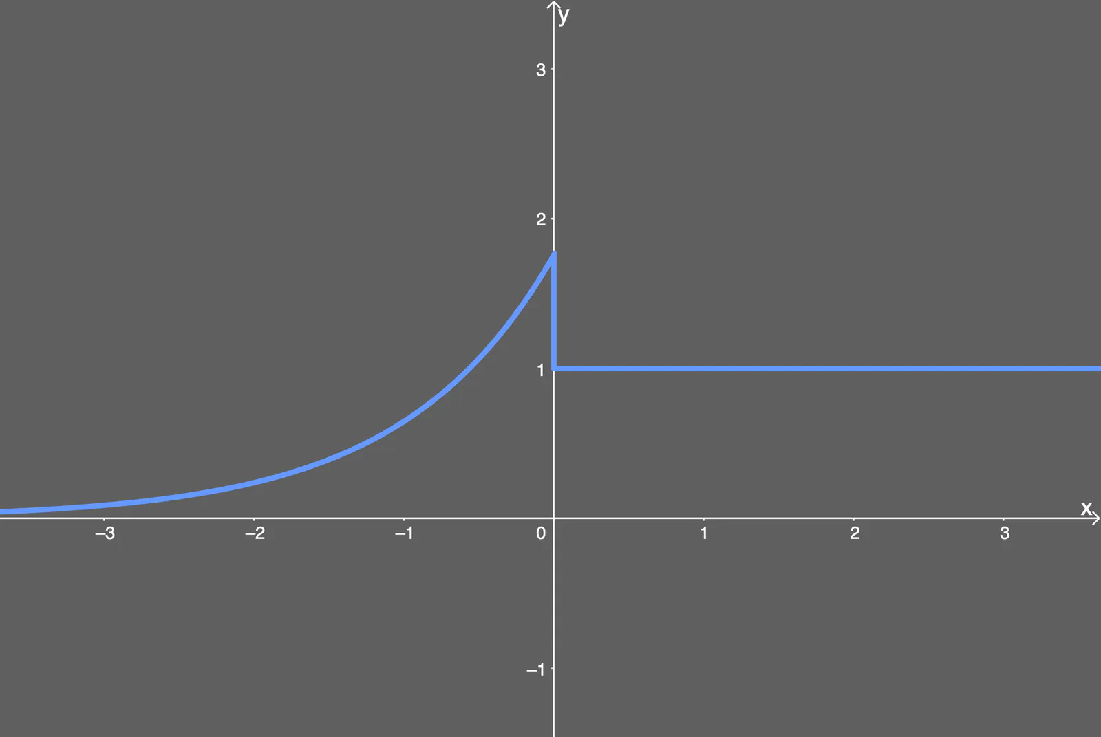
The SELU function differentiated

Note that the SELU function also requires a weight initialization method called LeCun Normal, and if you want to use dropout, you have to use a special version called Alpha Dropout.

Pros

• Internal normalization is faster than external normalization, which means the network converges faster.
• Vanishing and exploding gradient problem is impossible, shown by their theorems 2 & 3 in the appendix.

Cons

• Relatively new activation function – needs more papers on architectures such as CNNs and RNNs, where it is comparatively explored. One paper talks about CNNs with SELU here.

GELU

Gaussian Error Linear Unit. An activation function used in the most recent Transformers – Google's BERT and OpenAI's GPT-2. The paper is from 2016, but is only catching attention up until recently.

This activation function takes the form of this equation:

$$\text{GELU}(x) = 0.5x\left(1+\text{tanh}\left(\sqrt{2/\pi}(x+0.044715x^3)\right)\right)$$

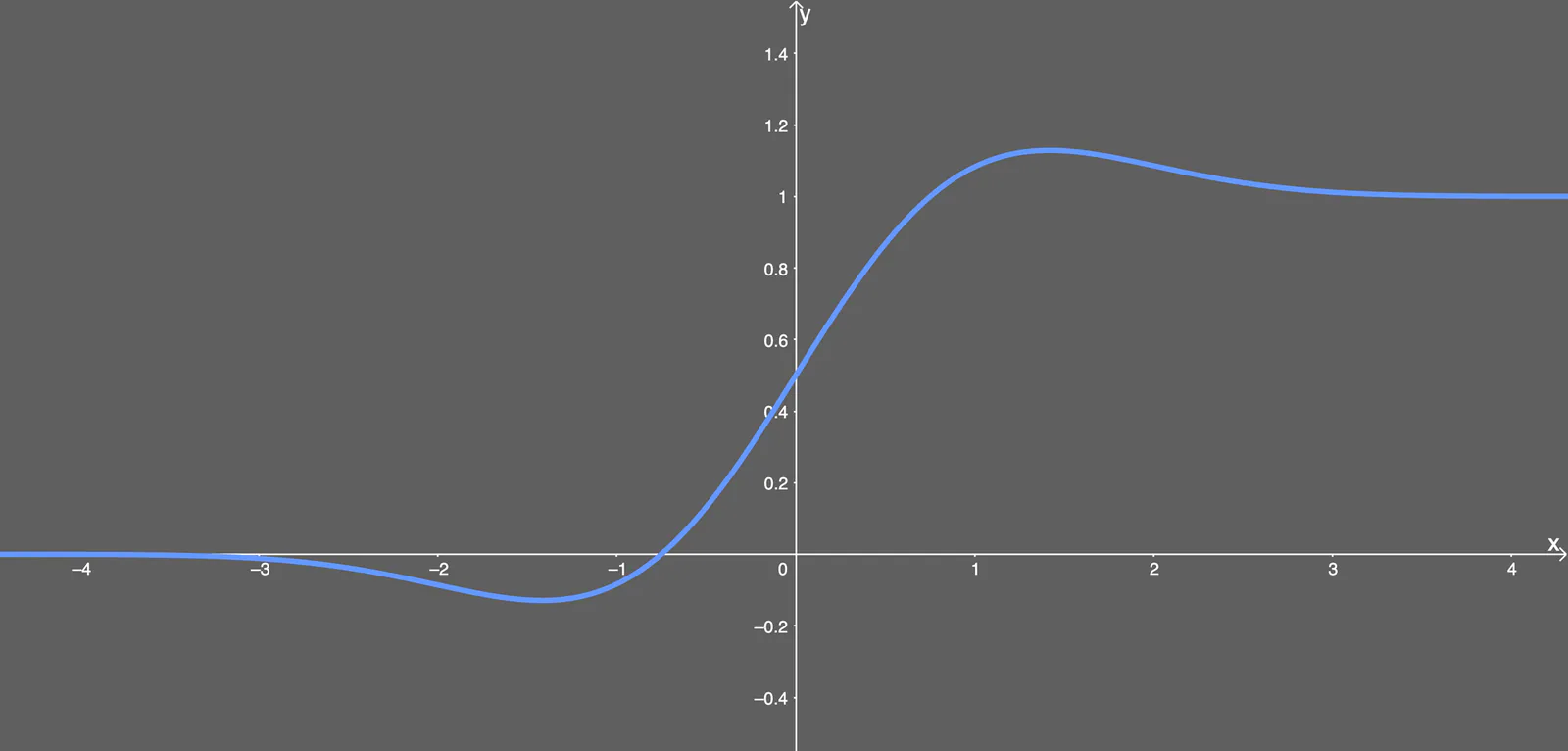
So it's just a combination of some functions (e.g. hyperbolic tangent tanh) and approximated numbers – there is not much to say about it. What is more interesting, is looking at the graph for the gaussian error linear unit:

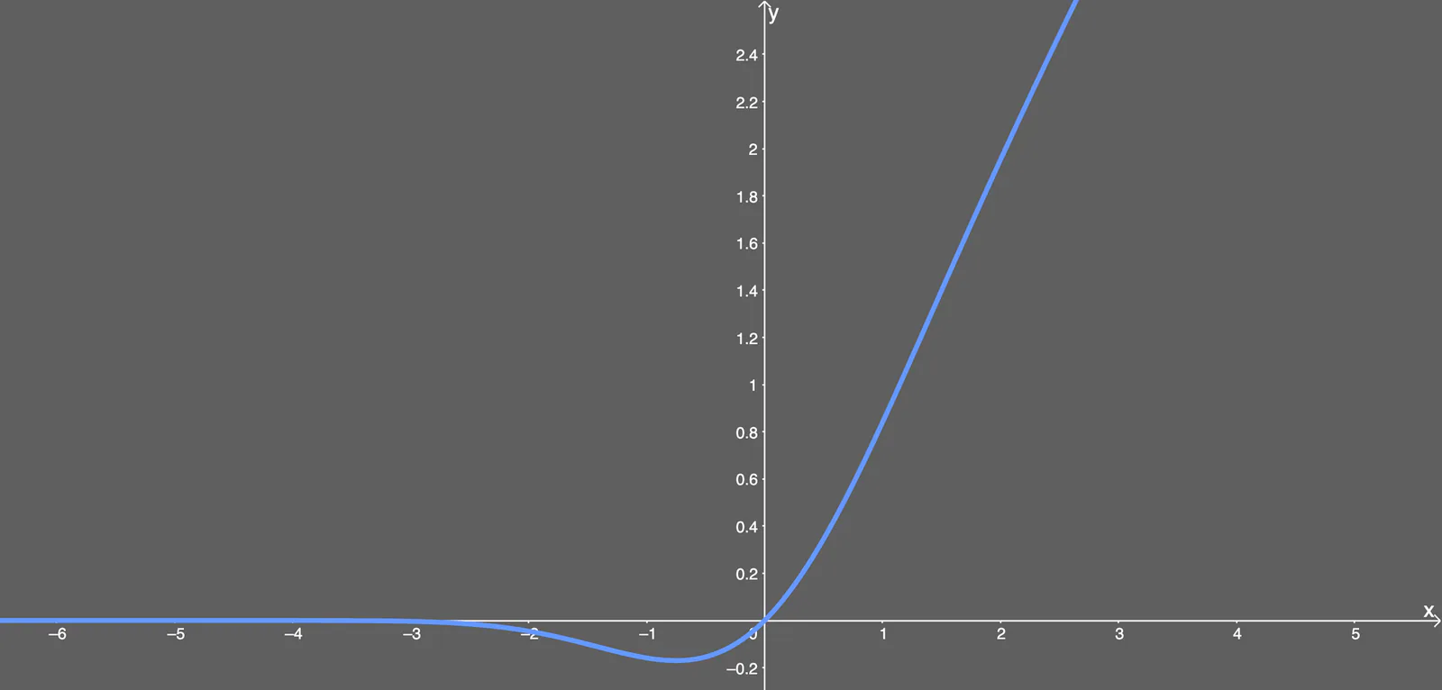
The GELU activation function

It has a negative coefficient, which shifts to a positive coefficient. So when $x$ is greater than zero, the output will be approximately $x$, except from when $x=0 \text{ to } x=1$, where it slightly leans to a smaller y-value.

I was unable to find the derivative anywhere, so naturally I turned to WolframAlpha and got it to differentiate the function. The result was this equation:

$$\text{GELU}'(x) = 0.5\text{tanh}(0.0356774x^3 + 0.797885 x) + (0.0535161 x^3 + 0.398942 x) \text{sech}^2(0.0356774x^3+0.797885x)+0.5$$

This is just another combination of hyperbolic functions as before. The plot of this function does look interesting though.

GELU activation function differentiated

Pros

• Seems to be state-of-the-art in NLP, specifically Transformer models – i.e. it performs best
• Avoids vanishing gradients problem

Cons

• Fairly new in practical use, although introduced in 2016.

Code For Deep Neural Networks

Let's say you want to try out all these activation functions, to find out which one is the best. How would you go about that? Usually we perform hyperparameter optimization – and this can be done using scikit-learn's GridSearchCV function. But we want to compare, so the idea is that we pick some hyperparameters and keep them constant, while changing the activation function.

Let me sketch for you, what I'm trying to do here:

1. Train the same neural network neural model over the activation functions mentioned in this post
2. Using the history for each activation function, make a plot of loss and accuracy over epochs.

This code was also published on GitHub with a colab button, so you can instantly run it for yourself; here is the link.

I prefer using the high-level API of Keras, so this is going to be done in Keras.

We start by importing everything we need. Note that 4 libraries are used here; tensorflow, numpy, matplotlib and keras.

import tensorflow as tf
import numpy as np
import matplotlib.pyplot as plt
from keras.datasets import mnist
from keras.utils.np_utils import to_categorical
from keras.models import Sequential
from keras.layers import Dense, Dropout, Flatten, Conv2D, MaxPooling2D, Activation, LeakyReLU
from keras.layers.noise import AlphaDropout
from keras.utils.generic_utils import get_custom_objects
from keras import backend as K
from keras.optimizers import Adam

From here, we would want to load a dataset to run this experiment on; let's choose the MNIST dataset. We can import it directly from Keras.

(x_train, y_train), (x_test, y_test) = mnist.load_data()

That's great, but we want to preprocess the data, as to normalize it. We do this by many functions, mainly we .reshape the images and divide by /= 255, the max RGB value. At last, we one-hot encode the data by to_categorical().

def preprocess_mnist(x_train, y_train, x_test, y_test):
    # Normalizing all images of 28x28 pixels
    x_train = x_train.reshape(x_train.shape[0], 28, 28, 1)
    x_test = x_test.reshape(x_test.shape[0], 28, 28, 1)
    input_shape = (28, 28, 1)
    
    # Float values for division
    x_train = x_train.astype('float32')
    x_test = x_test.astype('float32')
    
    # Normalizing the RGB codes by dividing it to the max RGB value
    x_train /= 255
    x_test /= 255
    
    # Categorical y values
    y_train = to_categorical(y_train)
    y_test= to_categorical(y_test)
    
    return x_train, y_train, x_test, y_test, input_shape
    
x_train, y_train, x_test, y_test, input_shape = preprocess_mnist(x_train, y_train, x_test, y_test)

Now that we have preprocessed the data, we are ready to build models and define some things for Keras to run. Let's start with the convolutional neural network model itself. For the SELU activation function, we have a special case, where we need to use a kernel initializer 'lecun_normal' and a special form of dropout AlphaDropout(), else everything is normal here.

def build_cnn(activation,
              dropout_rate,
              optimizer):
    model = Sequential()
    
    if(activation == 'selu'):
        model.add(Conv2D(32, kernel_size=(3, 3),
                  activation=activation,
                  input_shape=input_shape,
                  kernel_initializer='lecun_normal'))
        model.add(Conv2D(64, (3, 3), activation=activation, 
                         kernel_initializer='lecun_normal'))
        model.add(MaxPooling2D(pool_size=(2, 2)))
        model.add(AlphaDropout(0.25))
        model.add(Flatten())
        model.add(Dense(128, activation=activation, 
                        kernel_initializer='lecun_normal'))
        model.add(AlphaDropout(0.5))
        model.add(Dense(10, activation='softmax'))
    else:
        model.add(Conv2D(32, kernel_size=(3, 3),
                  activation=activation,
                  input_shape=input_shape))
        model.add(Conv2D(64, (3, 3), activation=activation))
        model.add(MaxPooling2D(pool_size=(2, 2)))
        model.add(Dropout(0.25))
        model.add(Flatten())
        model.add(Dense(128, activation=activation))
        model.add(Dropout(0.5))
        model.add(Dense(10, activation='softmax'))
    
    model.compile(
        loss='binary_crossentropy', 
        optimizer=optimizer, 
        metrics=['accuracy']
    )
    
    return model

We do have a small problem with the GELU function; it does not yet exist in Keras. Luckily for us, it's quite easy to add a new activation function to Keras.

# Add the GELU function to Keras
def gelu(x):
    return 0.5 * x * (1 + tf.tanh(tf.sqrt(2 / np.pi) * (x + 0.044715 * tf.pow(x, 3))))
get_custom_objects().update({'gelu': Activation(gelu)})

# Add leaky-relu so we can use it as a string
get_custom_objects().update({'leaky-relu': Activation(LeakyReLU(alpha=0.2))})

act_func = ['sigmoid', 'relu', 'elu', 'leaky-relu', 'selu', 'gelu']

Now we are ready to train the model using different activation functions, defined in the act_func array. We run a simple for-loop over each activation function, and add its results to an array

result = []

for activation in act_func:
    print('\nTraining with -->{0}<-- activation function\n'.format(activation))
    
    model = build_cnn(activation=activation,
                      dropout_rate=0.2,
                      optimizer=Adam(clipvalue=0.5))
    
    history = model.fit(x_train, y_train,
          validation_split=0.20,
          batch_size=128, # 128 is faster, but less accurate. 16/32 recommended
          epochs=100,
          verbose=1,
          validation_data=(x_test, y_test))
    
    result.append(history)
    
    K.clear_session()
    del model

print(result)

From this, we can plot the history that we got from our model.fit() for each activation function and have a look at how everything went.

Now we are ready to plot our data, and I made some short code using matplotlib

new_act_arr = act_func[1:]
new_results = result[1:]

def plot_act_func_results(results, activation_functions = []):
    plt.figure(figsize=(10,10))
    plt.style.use('dark_background')
    
    # Plot validation accuracy values
    for act_func in results:
        plt.plot(act_func.history['val_acc'])
        
    plt.title('Model accuracy')
    plt.ylabel('Test Accuracy')
    plt.xlabel('Epoch')
    plt.legend(activation_functions)
    plt.show()

    # Plot validation loss values
    plt.figure(figsize=(10,10))
    
    for act_func in results:
        plt.plot(act_func.history['val_loss'])
        
    plt.title('Model loss')
    plt.ylabel('Test Loss')
    plt.xlabel('Epoch')
    plt.legend(activation_functions)
    plt.show()

plot_act_func_results(new_results, new_act_arr)

This produces the graphs below

Further Reading

This is a GO-TO book that is practical and BEST in industry:

• Go purchase the BEST practical book
  Hands-On Machine Learning with Scikit-Learn and TensorFlow

Here are four books that are well-written:

• Deep Learning by Ian Goodfellow, Yoshua Bengio and Aaron Courville
• The Hundred-Page Machine Learning Book by Andriy Burkov
• Hands-On Machine Learning with Scikit-Learn and TensorFlow by Aurélien Géron
• Machine Learning: A Probabilistic Perspective by Kevin P. Murphy

Here are the papers, which were discussed in this article:

• Leaky ReLU paper
• ELU paper
• SELU paper
• GELU paper