Optimizers Explained - Adam, Momentum and Stochastic Gradient Descent

Picking the right optimizer with the right parameters, can help you squeeze the last bit of accuracy out of your neural network model.

October 16, 201917 min readUpdated Dec 19, 2019

Optimizers Explained - Adam, Momentum and Stochastic Gradient Descent

Picking the right optimizer with the right parameters, can help you squeeze the last bit of accuracy out of your neural network model. In this article, optimizers are explained from the classical to the newer approaches.

This post could be seen as a part three of how neural networks learn; in the previous posts, we have proposed the update rule as the one in gradient descent. Now we are exploring better and newer optimizers. If you want to know how we do a forward and backwards pass in a neural network, you would have to read the first part – especially how we calculate the gradient is covered in great detail.

If you are new to neural networks, you probably won't understand this post, if you don't read the first part.

Neural Networks: Feedforward and Backpropagation Explained
What are neural networks? Developers should understand backpropagation, to figure out why their code sometimes does not work. Visual and down to earth explanation of the math of backpropagation.
Casper Hansen · Machine Learning From Scratch

I want to add, before explaining the different optimizers, that you really should read Sebastian Ruder's paper An overview of gradient descent optimization algorithms. It's a great resource that briefly describes many of the optimizers available today.

Table of Contents (Click To Scroll)

Stochastic Gradient Descent
- Classical Algorithm and Code
Momentum Algorithm
Adam: Adaptive Moment Estimation
- Adaptive Learning Rate
  - AdaGrad: Sum of Gradients
  - RMSprop: Decaying Average
- Actually Explaining Adam
Further Readings

Stochastic Gradient Descent

This is the basic algorithm responsible for having neural networks converge, i.e. we shift towards the optimum of the cost function. Multiple gradient descent algorithms exist, and I have mixed them together in previous posts. Here, I am not talking about batch (vanilla) gradient descent or mini-batch gradient descent.

The basic difference between batch gradient descent (BGD) and stochastic gradient descent (SGD), is that we only calculate the cost of one example for each step in SGD, but in BGD, we have to calculate the cost for all training examples in the dataset. Trivially, this speeds up neural networks greatly. Exactly this is the motivation behind SGD.

The equation for SGD is used to update parameters in a neural network – we use the equation to update parameters in a backwards pass, using backpropagation to calculate the gradient $\nabla$ :

\theta = \theta - \eta \cdot \overbrace{\nabla_\theta J(\theta; \, x, \, y)}^{\text{Backpropagation}}

This is how the equation is presented formally, and here is what each symbol means:

$\theta$ is a parameter (theta), e.g. your weights and biases. Notice that we only update a single parameter for the neural network here, i.e. we could update a single weight.
$\eta$ is the learning rate (eta), but also sometimes alpha $\alpha$ or gamma $\gamma$ is used.
$\nabla$ is the gradient (nabla), which is taken of $J$ . Gradient calculations are already explained extremely well in my other post.
$J$ is formally known as objective function, but most often it's called cost function or loss function.

We take each parameter theta $\theta$ and update it by taking the original parameter $\theta$ and subtract the learning rate $\eta$ times the ratio of change $\nabla J(\theta)$ .

$J(\theta;\, x, \, y)$ just means that we input our parameter theta $\theta$ along with a training example and label (e.g. a class). The semicolon is used to indicate that the parameter theta $\theta$ is different from the training example and label, which are separated by a comma.

Note that moving forward, the subscript $\theta$ in $\nabla_\theta$ will be left out for simplicity.

We can visualize what happens to a single weight $w$ in a cost function $C(w)$ (same as $J$ ). Naturally, what happens is that we find the derivative of the parameter $\theta$ , which is $w$ in this case, and we update the parameter accordingly to the equation above.

If the gradient $\nabla$ of the partial derivatives is positive, we step left, else we step right when negative. GIF'ed from 3blue1brown video and added captions.

Okay, we got some value theta $\theta$ and eta $\eta$ to work with. But what is that last thing in the equation, what does it mean? Let's expand into the equation from the prior post (which you should have read).

\theta = \theta - \eta \cdot \nabla J(\theta; \, x, \, y) \Leftrightarrow \theta = \theta - \eta \cdot \frac{\partial C}{\partial \theta}

Well this is now just a partial derivative, i.e. we find the cost function $C$ , and inside that function, we find the derivative of theta $\theta$ , but keep the rest of the function constant (we don't touch the rest). The assumption here is that our training example with a label is provided, which is why it was removed on the right side.

We could even replace some of the terms to make it more readable. Say we wanted to update a weight $w$ , with the learning rate $0.3$ and a cost function C:

w = w - 0.3 \cdot \frac{\partial C}{\partial w}

Well, we assume that we know $w$ , so the only thing stopping us from calculating the equation is the last term. But I won't go into that, since that was part of my last post.

Moving forward, note and remember that

\nabla J(\theta) = \frac{\partial C}{\partial \theta}

If you don't know what this means, perhaps you should visit neural networks post, which in detail will explain backpropagation, and what gradients and partial derivatives mean.

Classical Algorithm and Code

For each parameter theta $\theta$ , from $1$ to $j$ , we update according to this equation.

\theta_j = \theta_j - \eta \cdot \overbrace{\frac{\partial C}{\partial \theta_j}}^{\text{Backprop}}

Usually, this equation is wrapped in a repeat until convergence, i.e. we update each parameter, for each training example, until we reach a local minimum.

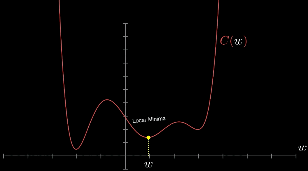
This is a local minimum.

Running through the dataset multiple times is usually done, and each pass through the dataset is called an epoch, and for each epoch, we should randomly shuffle the data – this is the stochasticity of the algorithm.

Say we want to translate this to some pseudo code. This is relatively easy, except for we will leave the function for calculating gradients left out.

for i in range(n_epochs):
    np.random.shuffle(data)  # shuffles in place
    for x,y in data:
        # Using backpropagation to calculate gradients (change)
        change = compute_gradient(cost_func, x, y, param)
        param = param - l_rate * change

Ending the walkthrough of SGD, it is only right to propose some pros and cons of the optimizer. Clearly, it is one of the older algorithms for optimization in neural networks, but nevertheless, it is also comparatively the easiest to learn. The cons are mostly with regards to newer and better optimizers, and is perhaps hard to explain at this point. The reason for the cons will become clear, once I present the next optimizers.

Pros

Relatively fast compared to the older gradient descent approaches
SGD is comparatively easy to learn for beginners, since it is not as math heavy as the newer approaches to optimizers

Cons

Converges slower than newer algorithms
Has more problems with being stuck in a local minimum than newer approaches
Newer approaches outperform SGD in terms of optimizing the cost function

Momentum

Simply put, the momentum algorithm helps us progress faster in the neural network, negatively or positively, to the ball analogy. This helps us get to a local minimum faster.

Motivation for momentum

For each time we roll the ball down the hill (for each epoch), the ball rolls faster towards the local minimum in the next iteration. This makes us more likely to reach a better local minimum (or perhaps the global minimum) than we could have with SGD.

When optimizing the cost function for a weight, we might imagine a ball rolling down a hill amongst many hills. We hope that we get to some form of optimum.

The slope of the cost function is not actually such a smooth curve, but it's easier to plot to show the concept of the ball rolling down the hill. The function will often be much more complex, hence we might actually get stuck in a local minimum or significantly slowed down. Obviously, this is not desirable. The terrain is not smooth, it has obstacles and weird shapes in very high-dimensional space – for instance, the concept would look like this in 2D:

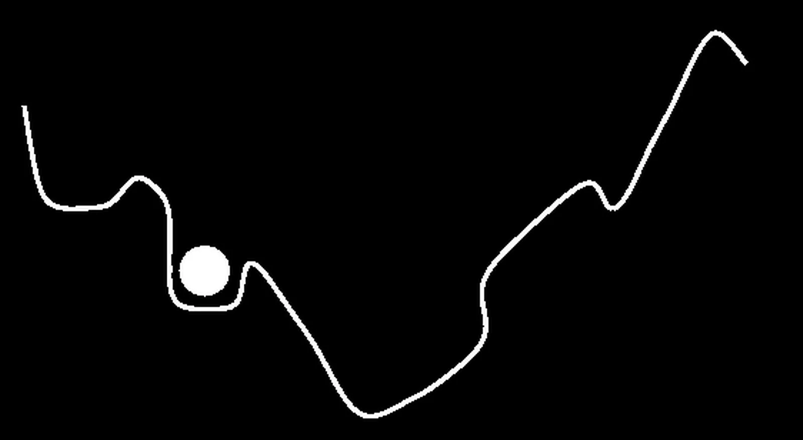
Ball stuck on a hilly 2D curve. Tweaked image from Quora user

In the above case, we are stuck at a local minimum, and the motivation is clear – we need a method to handle these situations, perhaps to never get stuck in the first place.

Now we know why we should use momentum, let's introduce more specifically what it means, by explaining the mathematics behind it.

Explanation of momentum

Momentum is where we add a temporal element into our equation for updating the parameters of a neural network – that is, an element of time.

This time element increases the momentum of the ball by some amount. This amount is called gamma $\gamma$ , which is usually initialized to $0.9$ . But we also multiply that by the previous update $v_t$ .

What I want you to realize is that our function for momentum is basically the same as SGD, with an extra term:

\theta = \theta - \eta\nabla J(\theta) - \gamma v_{t}

Let's just make this $100\%$ clear:

Theta $\theta$ is a parameter, e.g. your weights or biases
Eta $\eta$ is your learning rate, also sometimes written as alpha $\alpha$ or epsilon $\epsilon$ .
Objective function $J$ , i.e. the function which we are trying to optimize. Also called cost function or loss function (although they have different meanings).
Gamma $\gamma$ , a constant term. Also called the momentum, and rho $\rho$ is also used instead of $\gamma$ sometimes.
Last change (last update) to $\theta$ is called $v_t$ .

Although it's very similar to SGD, I have left out some elements for simplicity, because we can easily get confused by the indexing and notational burden that comes with adding temporal elements.

Let's add those elements now. First the temporal element, then the explanation of $v_t$ .

If you want to play with momentum and learning rate, I recommend visiting distill's page for Why Momentum Really Works.

Adding Time Steps $t$

We clearly see, that as we increase momentum, we get to the local minimum faster, but we might also overshoot and then it takes longer.

Adding the notion of time; say we want to update the current parameter $\theta$ , how would we go about that? Well, we would first have to define which parameter $\theta$ we want to update at a given time. And how do we do that?

One way to track where we are in time, is to assign a variable of time $t$ to $\theta$ . The variable $t$ would work like a counter; we increase $t$ by one for each update of a certain parameter.

How might this look in a mathematical sense? Well, we just subscript every variable that is subject to change over time. That is, the values for our parameter $\theta$ will definitely change over time, but the variable for the learning rate $\eta$ remains fixed.

\theta_{t+1} = \theta_{t} - \eta\nabla J(\theta_{t}) - \gamma v_{t}

This reads:

Theta $\theta$ at time step $t+1$ equals $\theta_t$ minus the learning rate, times the gradient of the objective function $J$ with respect to the parameter $\theta_t$ , minus a momentum term gamma $\gamma$ , times the change to $\theta$ at the last time step $t-1$ .

There it is, we added the temporal element. But we are not done, what does $v_t$ mean? I explained it as the previous update, but what does that entail?

Momentum Term

I told you about the ball rolling faster and faster down the hill, as it accumulates more speed for each epoch, and this term helps us do exactly that.

What helps us accumulate more speed for each epoch is the momentum term, which consists of a constant $\gamma$ and the previous update $v_{t}$ to $\theta$ . But the previous update to $\theta$ also includes the second last update to $\theta$ (scaled down by $\gamma$ ) and so on.

v_{t} = \eta\nabla J(\theta_{t-1}) + \gamma v_{t-1}

Essentially, we store the calculations of the gradients (the updates) for use in all the next updates to a parameter $\theta$ . This exact property causes the ball to roll faster down the hill, i.e. we converge faster because now we move forward faster.

Instead of writing $v_{t-1}$ , which includes $v_{t-2}$ in its equation and so on, we could use summation, which might be more clear. We can sum from tau $\tau$ equal to $1$ , all the way up to the previous time step $t-1$ . Notice that older gradients are multiplied by higher powers of $\gamma$ , so their influence decays over time.

\theta_{t+1} = \theta_{t} - \eta\nabla J(\theta_{t}) - \sum_{\tau=1}^{t-1} \gamma^{t-\tau} \eta\nabla J(\theta_{\tau})

The intuition of why momentum works (besides the theory) can effectively be shown with a contour plot – which is a long and narrow valley in this case.

The gist of momentum is that we get to the local minimum faster, because we don't oscillate up and down the y-axis. The time to convergence is faster when using momentum, but the animation is made equally long for a comparison of steps needed.

We can think of optimizing a cost function with SGD as oscillating up and down along the y-axis, and the bigger the oscillation up and down the y-axis, the slower we progress along the x-axis. Intuitively, it then makes sense to add something (momentum) to help us oscillate less, thus moving faster along the x-axis towards the local minimum.

\updownarrow \text{slower convergence}\\ \leftrightarrow \text{faster convergence}

The next notation for the notion of change might be more explainable and easier to understand. You may skip the next header, but I think it's a good alternative way of thinking about momentum. You will learn a different notation, which can enable you to understand other papers using similar notation.

Different Notation: A second explanation

In the paper that I linked at the start of the momentum section, it's described in a similar way but with different notation, so let's just cover that as well. They defined it for a weight instead of a parameter $\theta$ , and they use $E$ for error function, which is the same as $J$ for objective or cost function. They also use the Delta symbol $\Delta$ to indicate change:

\Delta w_t = \epsilon \nabla E(w) + \rho \Delta w_{t-1}

This is pretty straight forward, so let's replace the parameters of the equation with the parameters of what I just explained.

$w_t$ becomes $\theta_t$
$E(w)$ becomes $J(\theta_{t})$
Rho $\rho$ becomes $\gamma$

Rewriting the parameters, we get almost the same exact equation as presented in the last notation, except we now have a Delta $\Delta$ term at the start and end of the equation. Intuitively, the delta symbol has always meant change when studying physics – and it has the same meaning here, it's just some rate of change for a parameter over a function $J$ .

\Delta \theta_t = \eta \nabla J(\theta_t) + \gamma \Delta \theta_{t-1}

All the triangle delta means can be specified as a function $\text{change}(\theta_t)$ , which just specifies how much a parameter $\theta$ should change by. So when I tell you that I want you to add $\Delta \theta_{t-1}$ at the end of the equation, it just means to take the last change to $\theta$ , i.e. at the last time step $t-1$ .

Now $\Delta \theta_t$ becomes our update, and we update our parameter accordingly:

\theta_{t+1} = \theta_t - \Delta \theta_t

It's really that simple.

There is not much to say for pros and cons of the algorithm – perhaps there is not too much theory on the subject of the good and bad of momentum.

Pros

Faster convergence than traditional SGD

Cons

As the ball accelerates down the hill, how do we know that we don't miss the local minimum? If the momentum is too much, we will most likely miss the local minimum, rolling past it, but then rolling backwards, missing it again. If the momentum is too much, we could just swing back and forth around the local minimum.

Adam

Adaptive Moment Estimation (Adam) is the next optimizer, and probably also the optimizer that performs the best on average. Taking a big step forward from the SGD algorithm to explain Adam does require some explanation of some clever techniques from other algorithms adopted in Adam, as well as the unique approaches Adam brings.

Adam uses Momentum and Adaptive Learning Rates to converge faster. We have already explored what Momentum means, now we are going to explore what adaptive learning rates mean.

Comparison of many optimizers. Credits to Ridlo Rahman

Adaptive Learning Rate

An adaptive learning rate can be observed in AdaGrad, AdaDelta, RMSprop and Adam, but I will only go into AdaGrad and RMSprop, as they seem to be the relevant ones (although AdaDelta has the same update rule as RMSprop). The adaptive learning rate property is closely related to Learning Rate Schedules, which I found an insightful Medium post for.

So, what is it? I found that the best way is explaining a property from AdaGrad first, and then adding a property from RMSprop. This will be sufficient to show you what adaptive learning rate means and provides.

Part of the intuition for adaptive learning rates, is that we start off with big steps and finish with small steps – almost like mini-golf. We are then allowed to move faster initially. As the learning rate decays, we take smaller and smaller steps, allowing us to converge faster, since we don't overstep the local minimum with as big steps.

AdaGrad: Parameters Gets Different Learning Rates

Adaptive Gradients (AdaGrad) provides us with a simple approach, for changing the learning rate over time. This is important for adapting to the differences in datasets, since we can get small or large updates, according to how the learning rate is defined.

Let's go for a top to bottom approach; here is the equation:

\theta_{t+1,i} = \theta_{t,i} -\frac{\eta} { \sqrt { \epsilon + \sum_{\tau=1}^{t} \left( \nabla J(\theta_{\tau,i}) \right) ^2 } } \nabla J(\theta_{t,i})

All we added here is division of the learning rate eta $\eta$ . Although I told you that $\epsilon$ sometimes is the learning rate, in this algorithm it is not. In fact, it's just a small value that ensures that we don't divide by zero.

What needs explaining here is the term $\sqrt{\sum_{\tau=1}^{t}\left( \nabla J(\theta_{\tau,i}) \right) ^2}$ , i.e. the square root of the summation $\sum$ over all gradients squared. We sum over all the gradients, from time step $\tau=1$ all the way to the current time step $t$ .

If $t=3$ , then we would sum over the gradient at $t=1$ , $t=2$ and $t=3$ , and this just scales as $t$ becomes larger. Eventually, though, the sum might be so large, that the effective learning rate becomes stale, i.e. it updates with very small values.

Let me just make an example here, denoting the gradient by $g$ under the square root, i.e. $g(\theta_{3,i})^2 = (\nabla J(\theta_{3,i}))^2$

\theta_{4,i} = \theta_{3,i} \, -\frac{\eta} { \sqrt { \epsilon + g(\theta_{1,i})^2 + g(\theta_{2,i})^2 + g(\theta_{3,i})^2 } } \,\nabla J(\theta_{3,i})

What effect does this have on the learning rate $\eta$ ? Well, division by bigger and bigger numbers means that the learning rate is decreasing over time – hence the term adaptive learning rate.

We could in simple terms say, that the sum $\sum$ increases over time, as we add more gradients over time:

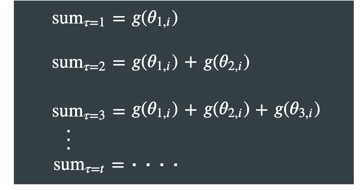
Overview of how the sum grows, as $t$ gets larger (the squares on each $g$ are left out of the picture for brevity).

RMSprop

Root Mean Squared Propagation (RMSprop) is very close to Adagrad, except for it does not provide the sum of the gradients, but instead an exponentially decaying average. This decaying average is realized through combining the Momentum algorithm and Adagrad algorithm, with a new term.

An important property of RMSprop is that we are not restricted to just the sum of the past gradients, but instead we are more restricted to gradients for the recent time steps. This means that RMSprop changes the learning rate slower than Adagrad, but still reaps the benefits of converging relatively fast – as has been shown (and we won't go into those details here).

Doing the top to bottom approach again, let's start out with the equation. By now, you should only be suspicious of the expectation of the gradient $E[g^2]$ :

\theta_{t+1,i} = \theta_{t,i} -\frac{\eta} { \sqrt { \epsilon + E[g^2]_t } } \nabla J(\theta_{t,i})

This exact term is what causes the decaying average (also called running average or moving average). Let's examine it, with relation to the momentum algorithm presented earlier.

Momentum:

\theta_{t+1} = \theta_t - \eta \nabla J(\theta_t) - \gamma v_t \\ \text{where} \\ v_t = \eta \nabla J(\theta_{t-1})+\gamma v_{t-1}

New Term $E$ :

E[g^2]_t=(1-\gamma)g^2 + \gamma E[g^2]_{t-1} \\ \text{where} \\ g = \nabla J(\theta_{t,i})

We still have our momentum term $\gamma=0.9$ . We can immediately see that the new term $E$ is similar to $v_t$ from Momentum; the difference is that $E$ has no learning rate in the equation, while it has added a new term $(1-\gamma)$ in front of the gradient $g$ . Note that summation $\sum$ is not used here, since it would involve a more complex equation. I tried to convert it, but got stuck because of the new term, hence I found it's not worth it to try and express it with a summation sign.

With the AdaGrad algorithm, the effective learning rate was monotonically decreasing, while in RMSprop, $\eta$ can adapt up and down in value, as we step further down the hill for each epoch. This concludes adaptive learning rate, where we explored two ways of making the learning rate adapt over time. This property of adaptive learning rate is also in the Adam optimizer, and you will probably find that Adam is easy to understand now, given the prior explanations of other algorithms in this post.

Andrew Ng compares Momentum to RMSprop in a brilliant video on YouTube

Momentum (blue) and RMSprop (green) convergence. We see that RMSprop is faster.

Actually Explaining Adam

Now we have learned all these other algorithms, and for what? Well, to be able to explain Adam, such that it's easier to understand. By now, you should know what Momentum and Adaptive Learning Rate mean.

There are a lot of terms to watch out for in the original paper, and it might seem confusing at first.

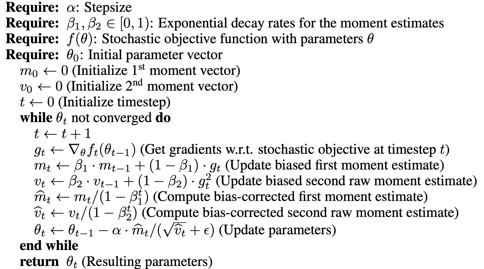
Adam algorithm in one picture in pseudo code. Taken from the original Adam paper.

But let's just paint it in a simplistic way; here is the update rule for Adam

\theta_{t+1} = \theta_t - \frac{\eta \cdot \hat{m_t}} { \sqrt{\hat{v_t}} + \epsilon } \\ \text{where} \\\\ \hat{m_t} = \frac{m_t}{1-\beta_1^t} \\ \hat{v_t} = \frac{v_t}{1-\beta_2^t} \\ \text{and where} \\ m_t = (1-\beta_1)g_t + \beta_1 m_{t-1} \\ v_t = (1-\beta_2)g_t^2 + \beta_2 v_{t-1}

Immediately, we can see that there are a bunch of numbers and things to keep track of. Most of these have already been explained, but for the sake of clarity, let's state each term here:

Epsilon $\epsilon$ , which is just a small term preventing division by zero. This term is usually $10^{-8}$ .
Learning rate $\eta$ (although it's $\alpha$ in the paper). They explain that a good default setting is $\eta=0.001$ , which is also the default learning rate in Keras.
The gradient $g$ , which is still the same thing as before: $g = \nabla J(\theta_{t,i})$

We also have two decay terms, also called the exponential decay rates in the paper. The terms are close to $\gamma$ in RMSprop and Momentum, but instead of 1 term, we have two terms called beta 1 and beta 2:

First momentum term $\beta_1=0.9$
Second momentum term $\beta_2=0.999$

Although these terms are without the time step $t$ , we would just take the value of $t$ and put it in the exponent, i.e. if $t=5$ , then $\beta_1^{t=5}=0.9^5=0.59049$ .

A Final Note

The likes of RAdam and Lookahead were considered, along with a combination of the two, called Ranger, but ultimately left out. They are acclaimed SOTA optimizers by a bunch of Medium posts, though they stand unproven. A future post could include these "SOTA" optimizers, to explain the difference from Adam, and why that might be useful.

Anyone getting into deep learning will probably get the best and most consistent results using Adam, as that has already been out there and shown that it performs the best.

If you want to visualize optimizers, I found this notebook to be a great resource, using optimizers from TensorFlow.