Principal Component Analysis (PCA) and Singular Value Decomposition (SVD)

This post will keep us on the level of Machine Learning Introduction, but it will try to give a clearer image of what happens behind, i.e. what PCA and SVD do.
Psst.. just want the algorithm (code), click here.

What is Principal Component Analysis (PCA)?

There is quite a lot of terminology from Linear Algebra in PCA, I will try to simplify these terms and give you an intuitive understanding, then show you those simple terms in Linear Algebra terms. I do suggest reading my Linear Algebra series before reading this, unless you already have the qualifications.

PCA is about projecting (Dot Product) data points onto a line, i.e. data points are projected into a lower dimension. PCA is a projection such that the variance in that projection is as high as possible. PCA is just finding the projection such that most of the variance of the data is accounted for.

[1] Moving Coordinate System

The first thing in a PCA is a sort of shift of the data onto a new coordinate system. You do this by calculating the mean for every dimension of your data, then subtracting the mean from every observation in that dimension. More loosely speaking, you calculate the mean feature by feature and subtract the mean from each observation for each feature.

In mathematical terms, this is known as centering the data by subtracting the mean — a translation of the coordinate system (note that it is not a Linear Transformation as covered here, since it moves the origin). $\widetilde{X}$ (X tilde) is just the new X, and X is all of our observations, while $\mu$ (mu) is the mean:

$$\widetilde{X} = X - \mu$$

The origin of our coordinate system would now have been shifted to the center of our data.

Here is the unintuitive way of calculating the mean and how you might have been presented with calculating the mean:

$$\mu = \frac{1}{n}\sum\limits^{n}_{i=1}x_i$$

But what it really says is just, sum all observations (add all observations together), then divide them by $n$, the number of observations. We call the result $\mu$ (mu), which is what we use in the formula for moving the coordinate system.

[2] Finding Principal Components

Now that we are at the center of our data, the objective would be to find the direction in which we get the most variance (imagine a line through origin and the data points). What is the most variance? It's just a fancy way of saying that we want the directions where there are most data points covered (e.g. by drawing a line in that direction).

Another way to look at variance is through a mathematical scope. Suppose we were to draw a line through our origin and our data points, how could we project each data point onto that line? And after projected, what is the distance to origin? What we really want is the line, after having projected all data points, where we have maximized the sum of the squared distances from all points to origin. That is what most variance is. So for each data point, we would have a distance d and we would have n data points, so we would sum all of the squared distances and divide them by $n-1$:

$$\frac{d_1^2+d_2^2+...+d_n^2}{n-1} = variance$$

Suppose we have that the variance along Principal Component 1 (PC1) is equal to 18 and along PC2 equal to 4, then the PC1 would account for $18/22 \approx 0.82=82\%$ and PC2 $4/22 \approx 0.18=18\%$. By the way, PC1 and PC2 are just the first and second principal component, corresponding to the principal component with the most variance and the principal component with the second most variance.

But how do you find such a line, that accounts for the most variance?

To answer this question, you would perhaps need a Linear Algebra background (read my Linear Algebra series 1-4).

The answer lies in something called Eigenvectors and Eigenvalues. So what is that, and how does it relate to PCA? All sorts of ideas are thrown around, like covariance matrix and all these other seemingly complex words that neither you nor I (before writing this) knew about. So what is it? Follow along.

Eigenvector and Eigenvalue Introduction

If I were to transfer Eigenvectors and Eigenvalues to something more familiar, you could say that eigenvectors follow along the lines of our standard basis vectors (though they are not the same), since eigenvectors are usually normalized to be unit vectors. What does this mean? Well, our standard basis vectors are usually of length (or magnitude) 1, which is exactly what a unit vector is. Similarly, we have scalars, which are comparable to eigenvalues. To sum it up, eigenvectors can be looked at through the scope of basis vectors, and eigenvalues are scalars.

---

To talk about eigenvectors and eigenvalues, I would need a few paragraphs and pictures to give you a clear understanding of what they are visually. Follow along if you have the time for that.

If we were to transform our vector space, wouldn't it be coincidental if we had a vector that only changes in length, but not direction? This is what we call an eigenvector. So any eigenvector is scaled in length, but does not change direction. The scaled length is what we refer to as the eigenvalue, namely just a scalar.

Let's take our basis vectors $\hat{i}$ and $\hat{j}$ into consideration. If we were to apply a shear, we could shift over $\hat{j}$ while $\hat{i}$ stays in place, making $\hat{i}$ an eigenvector with an eigenvalue of 1, meaning that the vector did not stretch nor squish. But it did stay in the same direction, making it an eigenvector.

The transformation would look like this, where the first matrix is the transformation we apply to the second matrix. The second matrix is just a way of writing up our basis vectors in a matrix, and that matrix is the left picture, while the result is the right picture:

$$\begin{bmatrix} 1 & 1 \\ 0 & 1 \end{bmatrix} \begin{bmatrix} 1 & 0 \\ 0 & 1 \end{bmatrix} = \begin{bmatrix} 1 & 1 \\ 0 & 1 \end{bmatrix}$$

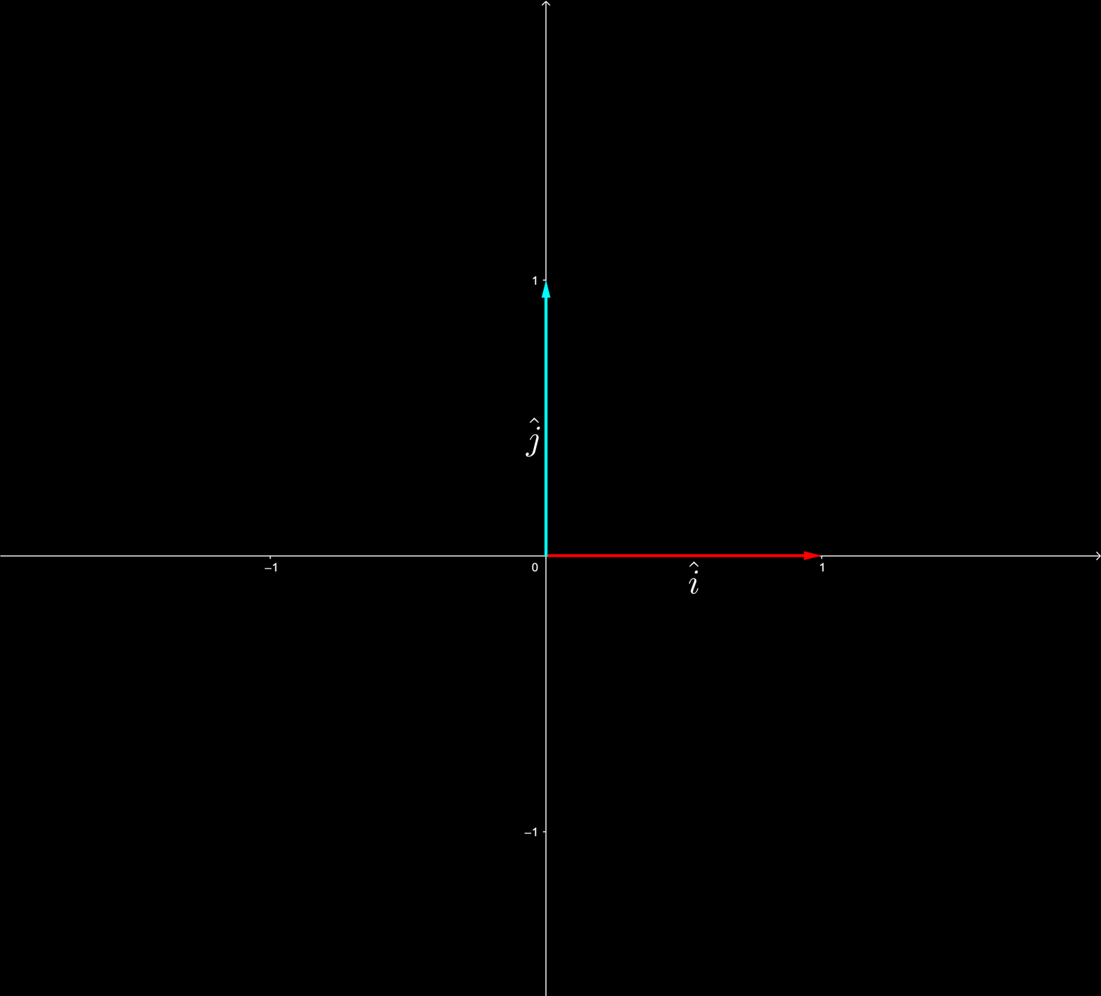
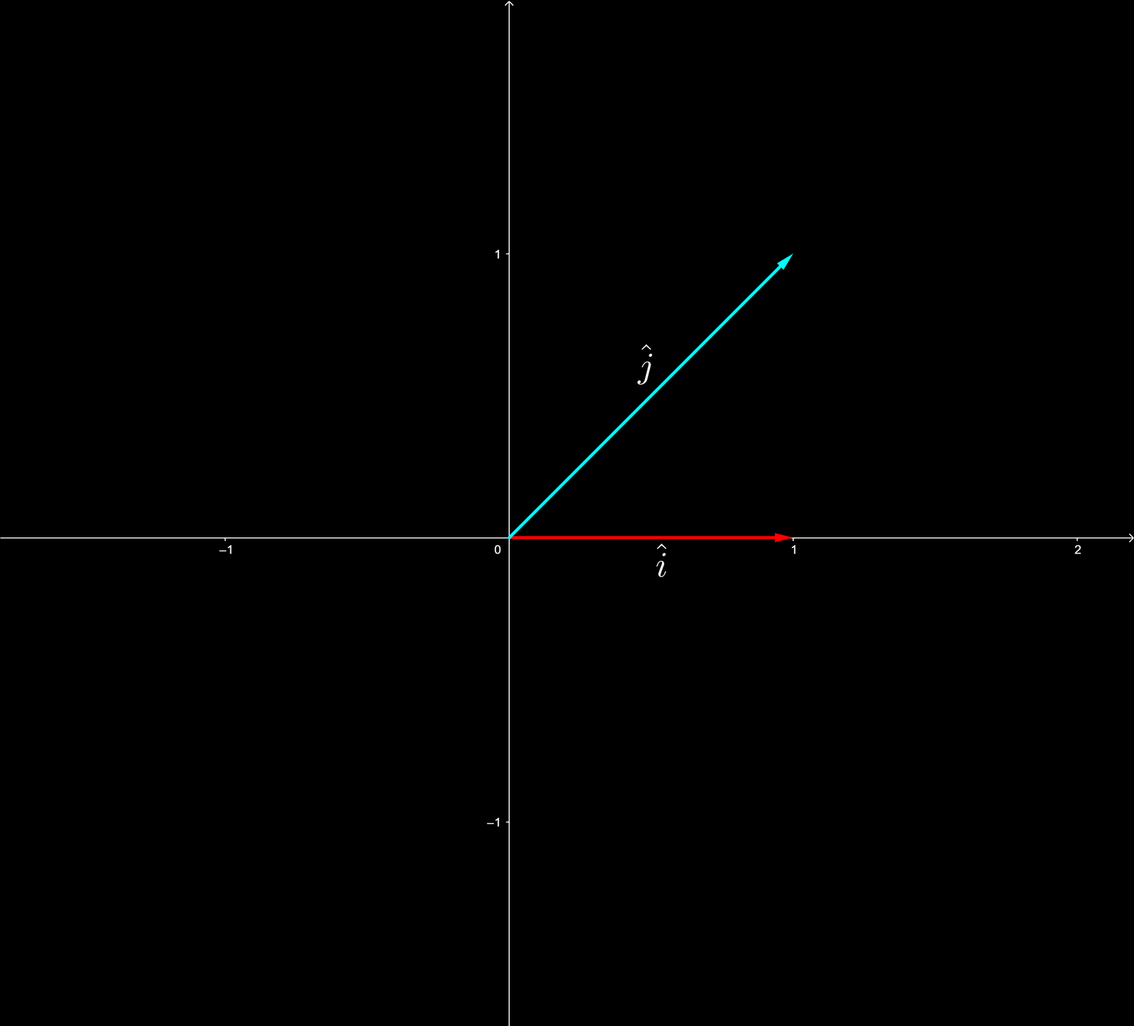
An example where $\hat{i}$ is an eigenvector with eigenvalue 1.

Finding the Eigenvectors and Eigenvalues

Now that we know what an eigenvector and eigenvalue is, let's take a deeper look at how we get the line that accounts for most variance for our data. This transformation represented above can help us gain an understanding of how to proceed with finding this line. With every transformation, there might or might not be eigenvectors, which is something we need to find out to do PCA. This is what we call an eigenvalue problem and here is the formula which you will be presented with everywhere:

$$A\vec{v}=\lambda \vec{v}$$

A is a transformation, a square matrix (the first matrix before the pictures), $\vec{v}$ is the eigenvector and $\lambda$ (lambda) is the eigenvalue. Most of the time, the literature will present or derive matrix A as

$$\widetilde{X}^T\widetilde{X}$$

Which I showed you parts of earlier. $\widetilde{X}$ (X tilde) is our data with the mean subtracted (so $\widetilde{X}^T\widetilde{X}$ is proportional to the covariance matrix), and the transpose (the T) flips any matrix so that it is the opposite. You just move the columns to rows and rows to columns

$$\begin{bmatrix} 1 & 2 \\ 3 & 4 \\ 5 & 6 \\ \end{bmatrix}^T = \begin{bmatrix} 1 & 3 & 5 \\ 2 & 4 & 6 \end{bmatrix}$$

---

The procedure for finding the line is

1. Finding the eigenvalue
2. Finding the eigenvector, using the eigenvalue

For the first step, what usually is represented is the formula here:

$$det(A-\lambda I)=0$$

If you read my Linear Algebra 4, you would know why we want to find the determinant equal to 0. It is because we will then have squished space into a lower dimension, which is what we want with PCA. We want to represent unimaginable data (100 dimensions) in a simple 2-dimensional plot.

I will take small parts from the first example here to show you how it could be done. The first thing to do is define A which they define as

$$A = \begin{bmatrix} 1 & -3 & 3 \\ 3 & -5 & 3 \\ 6 & -6 & 4 \end{bmatrix}$$

Then we want to form the matrix $A-\lambda I$

$$A-\lambda I = \begin{bmatrix} 1 & -3 & 3 \\ 3 & -5 & 3 \\ 6 & -6 & 4 \end{bmatrix} - \begin{bmatrix} \lambda & 0 & 0 \\ 0 & \lambda & 0 \\ 0 & 0 & \lambda \end{bmatrix} = \begin{bmatrix} 1-\lambda & -3 & 3 \\ 3 & -5-\lambda & 3 \\ 6 & -6 & 4-\lambda \end{bmatrix}$$

So the equivalent for this is just taking the original matrix A and subtracting $\lambda$ along the diagonal.

The next thing would be computing the determinant, which I'm going to cover very fast, since this is more of a computing part already covered in my Linear Algebra series. So the computation of the determinant looks like

$$det(A-\lambda I)=-\lambda^3 +12\lambda +16$$

This is what we end up with, but we are not done. We cannot solve any further, so we take the left side of the equation, set it equal to zero and switch every sign on both sides

$$\lambda^3 -12\lambda -16 = 0$$

Then we just solve for lambda (by computing) and get $\lambda = -2$ and $\lambda = 4$. We are not too concerned with how we get here, but the important part is that we ALWAYS pick the highest eigenvalue, because that is how we get the most variance. So we pick 4 as our eigenvalue. Our formula now looks like this:

$$\begin{bmatrix} 1 & -3 & 3 \\ 3 & -5 & 3 \\ 6 & -6 & 4 \end{bmatrix}\vec{v}=4 \vec{v}$$

Now it is step 2, finding the eigenvectors.

To find the eigenvectors, we would want to change up the formula. So we move everything from the right side of the formula to the left side and set it equal to 0:

$$A\vec{v}=\lambda \vec{v} \Longleftrightarrow (A-\lambda I)\vec{v}=0$$

Again, this is gone over fast here, so if we were to solve for this, we would find a resulting eigenvector for each eigenvalue. If you were to solve this, you would use Gaussian elimination.

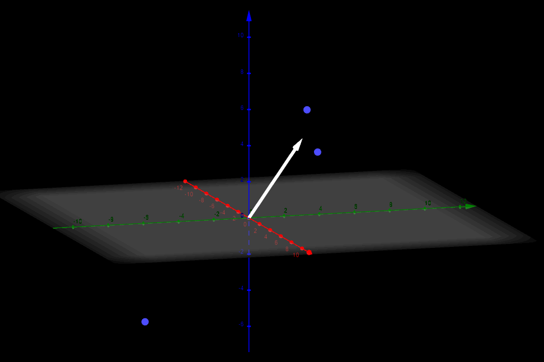
But let me just tell you, that the result for our highest eigenvalue of 4 is an eigenvector $\vec{v}=\begin{bmatrix}1 \\ 1 \\ 2 \end{bmatrix}$. If we plot the matrix A, as seen further up, we get these 3 data points. Then we can plot the eigenvector (also PC1) and let it be scaled by a variable amount. We can then see that it fits right in the middle of the data points, which will account for the most variance.

Here are three data points from the matrix A: $x_1=(1,3,6)$, $x_2=(-3,-5,-6)$ and $x_3=(3,3,4)$. Then there is the eigenvector, which is scaled by a variable amount. The eigenvector in this case is also PC1.

There we have it, that is PCA. The process is much simpler in terms of coding the algorithm, since there are premade libraries in Python and other programming languages, which you can just call.

What is Singular Value Decomposition (SVD)?

SVD is kind of the same as a PCA. So I'm going to keep it short, simple and non-mathematical.

So, SVD is similar to PCA. In PCA, you find the eigenvectors of $\widetilde{X}^T\widetilde{X}$, we just learned that. Now, what SVD does is to instead split the centered data matrix $\widetilde{X}$ itself into three matrices, $\widetilde{X} = USV^T$, without ever computing $\widetilde{X}^T\widetilde{X}$.

The columns of $V$ are unit vectors (vectors of length 1) that point in exactly the same directions as the eigenvectors from PCA — that is, they are the principal components. The values in $S$ are called singular values, and squaring them gives us the eigenvalues from before, i.e. how much variance each principal component accounts for.

The result is the same as with PCA, but SVD is numerically more stable and does not require forming the (possibly huge) matrix $\widetilde{X}^T\widetilde{X}$, which is why PCA is usually computed with SVD in practice — and that is exactly what the code further down does.

Why use PCA or SVD?

Well it really has just a few purposes, that maybe is not clear yet. PCA or SVD helps with dimensionality reduction, meaning that it takes m-dimensional data to a lower dimension than m, often to 2 or 3 dimensions, to represent the data there. So you really just find a lower dimensional representation of higher dimensional data.

It can be useful for

• Feature extraction, i.e. eliminating or suppressing parts of your data (obviously a small part, as PCA and SVD aim to keep a big percentage of the meaning of your data).
• Visualization, since you can't quite imagine a 100-dimensional dataset, but you can always plot a 2-dimensional dataset.
• General compression, it could be sound, video or image compression. PCA and SVD are quite efficient at performing lossy compression.

Algorithm

Let's look at how this is applied. The way you want to apply the SVD algorithmically, which is the one you normally choose to apply over PCA, is by these steps:

1. Subtract mean, move coordinate system to center of data.
2. Divide by standard deviation (standardizing the data). This step in particular means when we have encoded 1 feature to 10 features by one-hot encoding, those same features will tell us as much as 1 feature in a PCA. In other words it will have the same weight.
3. Compute SVD
4. Plot PCA

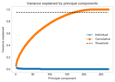
Here is a code piece, for a dataset that has been one-hot encoded from 76 to 272 columns (attributes).
Disclaimer: You cannot use this code, if you have any categorical data (features that are strings, like nationalities), without having one-hot encoded your data. I recommend using Pandas to do it train = pd.get_dummies(train, prefix_sep='_'). 'train' is your dataframe from Pandas and 'pd' is a reference to Pandas from the import below in this code.

# Data Manipulation
import numpy as np
import pandas as pd

# Visualization
import matplotlib.pyplot as plt
plt.style.use('seaborn-whitegrid')

# SVD Computation
from scipy.linalg import svd

# Get values from your dataframe (train)
# And get them from start to the range of columns
# (there are 272 columns)
X = train.get_values()[:,range(0,271)]

# Normalize data, subtract mean and divide by std
N = len(X)
Y = X - np.ones((N,1))*X.mean(axis=0)
Y = Y*(1/np.std(Y,0))

# compute the singular value decomposition with svd
U,S,V = svd(Y,full_matrices=False)

# Compute variance explained by principal components
rho = (S*S) / (S*S).sum()

# Set threshold for how much variance you at least want
threshold = 0.95

# Plot variance explained
# Magic
plt.figure()
plt.plot(range(1,len(rho)+1),rho,'x-')
plt.plot(range(1,len(rho)+1),np.cumsum(rho),'o-')
plt.plot([1,len(rho)],[threshold, threshold],'k--')
plt.title('Variance explained by principal components');
plt.xlabel('Principal component');
plt.ylabel('Variance explained');
plt.legend(['Individual','Cumulative','Threshold'])
plt.grid()
plt.show()

Here is the plot. Variance by principal component. To reach above 95% variance, we can tell that we need about 170 principal components. We do this by looking at the cumulative variance explained, which increases by cumulatively adding the variance from each component.